Evaporation II

Last week, we began exploring the piece Evaporation.  In particular, we looked at two aspects of the piece — randomness of both the colors and the sizes of the circles — and experimented with these features in Python.  Look at last week’s post for details!

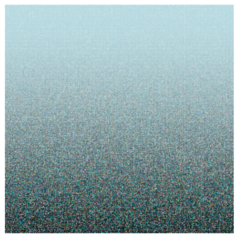
Today, we’ll examine the third significant aspect of the piece — the color gradient.  The piece is a pure sky blue at the top, but becomes more random toward the bottom.  How do we accomplish this?

Essentially, we need to find a way to introduce “0” randomness to each color at the top, and more randomness as we move toward the bottom.  To understand the concept, though, we’ll be introducing 0 randomness at the bottom, and more as we move up.  You’ll see why in a moment.

Let’s first look at a linear gradient.  Imagine that we’re working with a square — we can always scale later.  Here’s what it looks like:

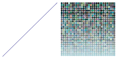
The “linear” part means we’re looking at randomness as a function of  So when we subtract randomness to each color.  But when we subtract a random number between and from each of the RGB values.  Finally, at the very top, we’re subtracting a random number between and from each RGB value.  Recall that if an RGB value would ever fall below as a result of subtraction, we’d simply treat the value as

Why do we subtract as we go up?  Recall that black has RGB values so subtracting the randomly generated number pushes the sky blue toward black.  If we added instead, this would push the sky blue toward white.  In fact, you can push the sky blue toward any color you want, but that’s a little too involved for today’s post.

The piece Evaporation was actually produced with a quadratic gradient.  Let’s look at a picture first:

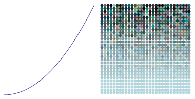
That the gradient is quadratic means that the randomness introduced is proportional to for each value of  In other words, at a level of on our square, we subtract a random number between and

You can visually see this as follows.  Look at the gradient of color change from to for the quadratic gradient.  This is approximately the same color change you see in the linear gradient between and  Why does this happen?  Because when you square numbers less than they get smaller.  So smaller numbers will introduce less randomness in a quadratic gradient than they will in a linear gradient.

We can go the other way, we well.  If we use a quadratic gradient (exponent of ), the color changes more gradually at the bottom.  But if we use an exponent less than (such as in taking a root, like a square root or cube root), we get the opposite effect:  color changes more rapidly at the bottom.  This is because taking a root of a number less than  increases the number.  It’s easiest to see this with an example:

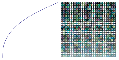
In this case, the exponent used is so that for a particular value, a random number between and is subtracted from each RGB value.  Note how quickly the color changes from the sky blue at the bottom toward very dark colors at the top.

Of course this is just one way to vary colors.  But I find it a very interesting application of power and root functions usually learned in precalculus — using computer graphics, we can directly translate an algebraic, functional relationship geometrically into a visual gradient of color.  Another example of why it is a good idea to enlarge your mathematical toolbox — you just never know when something will come in handy!  If I didn’t really understand how power and root functions worked, I wouldn’t have been able to create this visual effect so easily.

Now it’s your turn!  You can visit the Evaporation worksheet to try creating images on your own.  If you’ve been trying out the Python worksheets all along, the code should start to look familiar.  But a few comments are in order.

First, we just looked at a square.  It’s actually easier to think in terms of integer variables “width” and “height” (after all, there is no reason our image needs to be square).  In this case, we use “j” as the height parameter, since it is more usual to use variables like “i” and “j” for integers.  So “j/height” would correspond to  This would produce a color gradient of light to dark form bottom to top.

To make the gradient go from top to bottom, we use “(height-j)/height” instead (see the Python code).  This makes values near the top of the image correspond to and values near the bottom of the image correspond to  I’ll leave it to you to explore all the other details of the Python code.

Please feel free to comment with images you create using the Sage worksheet!

As mentioned in the previous post as well, each parameter you change — each number which appears anywhere in your code — affects the final image.  Some choices seem to give more appealing results than others.  This is where are meets technology.

As a final word — the work on creating fractals is still ongoing.  I’ve learned to make movies now using Processing:

You’ll notice how three copies of one fractal image morph into one of another.  You can find more examples on Twitter: @cre8math.  Once I feel I’ve had enough experience using Processing, I’ll post about how you can use it yourself.  The great thing about Processing is that you can use Python, so all your hard work learning Python will yield even further dividends!