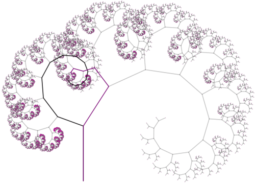
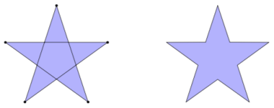
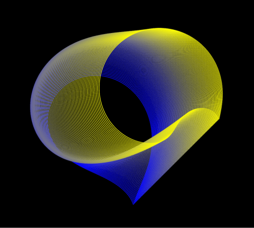
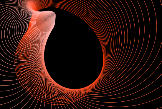
A few weeks, ago I dug out a problem which had puzzled me for over three years. I finally decided that now it was time to really dig in — and to my surprise and delight, not only did I solve the problem, but I’ve already got a draft of a paper written! The figure below is from that paper.

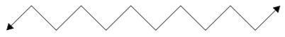
The problem is yet another variation on the recursion which produces the Koch snowflake. I discussed the Koch snowflake in one my first posts, so visit my Day007 post on this fascinating fractal for a refresher.
So what is the variation here? Consider the general recursive scheme

where 

The Koch curve is generated by choosing

Previously I’ve studied cases where 

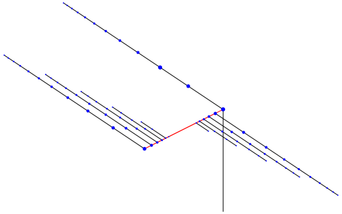
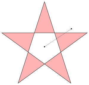
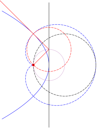
So let’s investigate the example illustrated above in more detail. The recursive scheme which generates this spiral is given by

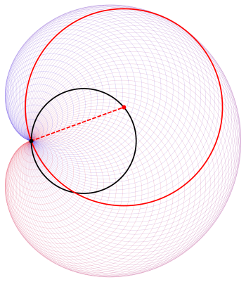
How does this scheme draw a spiral arm? Let’s look at the figure below.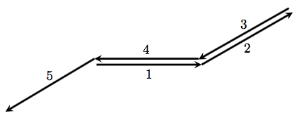
We begin at the origin, and then draw a segment at 


The next turn is 

What next? It is at this point that we invoke a recursive call — and so the next angle tells us what direction the next arm will be drawn in. Of course, like before, the three angles after that will continue drawing the arm and then bring us back to the origin, awaiting the next recursive call.
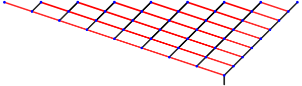
This behavior can be illustrated in the following chart.
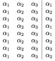
Here, the angles turned are listed in rows of four, one after another. The first three angles in each row are the same, and their job is to complete the arm once a direction is chosen. But the direction chosen is determined by the fourth column (separated by the divider), whose behavior is not periodic and highly recursive.
So where do we go from here? The next chart we’ll look it is a chart of the directions the arms are drawn in.
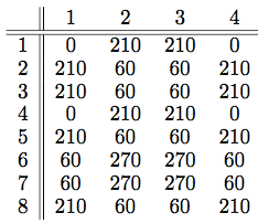
We read this chart in rows as follows: the first arm is drawn at an angle of 
But the third arm exactly retraces the second arm drawn, since it is pointed in the direction of 

So you can see what’s going on. One important consequence of the recursive algorithm is that the arms keep being retraced over and over again.
When will the complete spiral be drawn? Well, we need to see every multiple of
How would you show this? We can’t go into all the details here. The important observation is that if you read across the chart one row at a time, you get the same sequence of angles by reading down the first column of the chart.
But it isn’t enough to just observe this — it has to be proved. This is where some elementary number theory comes in. No more than what might be seen in an undergraduate number theory course, but beyond the scope of this post.
Slight step up on my soapbox — while I usually deplore the definition of mathematics as the “science of finding patterns” (as this only scratches the surface), in this case, finding patterns is critically important. With some trial and error, you hit upon making charts in rows of four, and then putting the directions the arms are drawn in rows of four, and then stare at the numbers until you notice patterns in the charts. The trick is knowing what to prove — once stated properly, the results almost prove themselves.
You’ll have to wait for the paper to come out for all the details. But here is a brief summary. Suppose you divide the circle into n parts, where n is even. Then devise a recursive scheme using the turning angles

Now define
When n is divisible by 4, the spiral has n arms, and you need to draw exactly 
But when n is even but not divisible by four, the spiral only has n/2 arms, and it takes 
Absolutely amazing, in my opinion. I formulated these conjectures over three years ago, but got stuck. A few weeks ago I had the house to myself for a while, and I just sat down and said to myself, “Look, you’ve already written one paper on these recursions. You can do this.”
And within two days, I worked out the patterns. Then the proofs, and within a week, a draft of the paper.
I am always humbled by such a seemingly innocuous problem — generating a simple spiral . But there are so many levels to this problem, and so much interesting mathematics to be discovered. I’ll continue exploring recursively drawn images, and share the amazing results with you when I find them!
 as an angle exterior to
  The analysis of all the other cases builds from this.
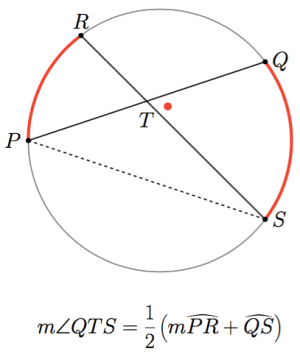
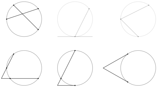
 moves around the circle. While, as mentioned, this cannot be addressed rigorously, it is a very intuitive argument. Moreover, there are many different software packages you could use to make an animation of this process, and display all the arc and angle measurements as
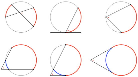

 and
and  eventually reach 0, you’re not able to conclude anything about a relationship between
  and
and 


 and
and  then
then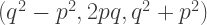
 for example, using this parameterization. Of course
  is just three times the triple
  therefore, if you can generate all primitive Pythagorean Triples, you can take multiples of them to generate all Pythagorean Triples.
 has side lengths which are in arithmetic progression. What other Pythagorean Triples have this property?
 where
where  is the smallest integer in the arithmetic progression and
  is the common difference. Since the triangle is a right triangle, we must have


 or
or  We did assume that
  so we eliminate the solution
  Note that this would generate the triple
  and in fact
  But one side length is zero and another is negative, so no triangle is possible with these side lengths.
 ? Here, we get
 of the primitive Pythagorean Triple
 right triangle.
 triangle, the area and perimeter were both
  A coincidence? Were there other triangles with this property?
 is necessary since the two-variable version generates all primitive Pythagorean Triples, but not necessarily all Pythagorean Triples.

 results in
 and the other two factors must be
 then
then  so that
  Substituting back into the parameterization, we obtain the Pythagorean Triple
  which is the triple
 then
then  so that
  This generates a new Pythagorean Triple,
 then
then  and
and  so that the Pythagorean Triple
  is generated. Of course this is just a duplicate of the first solution.
 and that their perimeters are equal. Prove that the triangles are congruent.
 where it crosses the x-axis at
  we simply retain the
  term and substitute the root
  into the other terms, getting

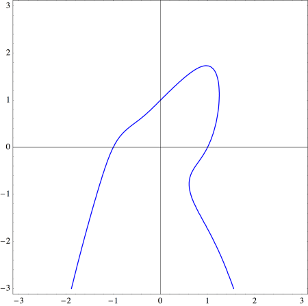
 (the U-shaped piece, since the sideways U-shaped piece involves writing
  as a function of
  ) is
) is  as shown below.
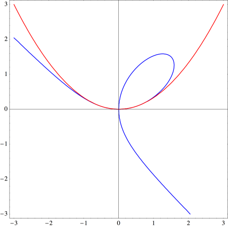

 and so rewrite the equation for the Folium of Descartes by using the substitution
  which results in
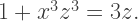
 we have
  giving us a good quadratic approximation at the origin.
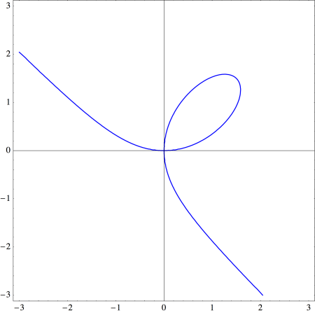
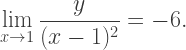
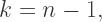
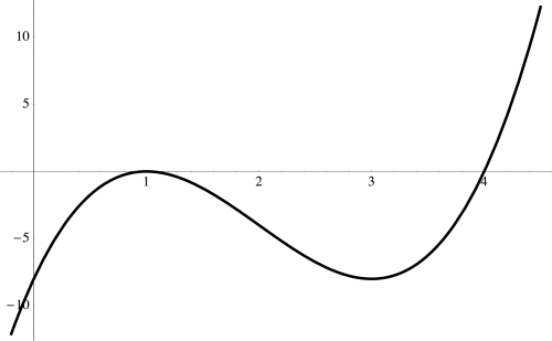
 looking at the curve

 with
with 
 we have
 Thus, in our case with
  we see that
  is a good approximation to the curve near the origin. The graph below shows just how good an approximation it is.
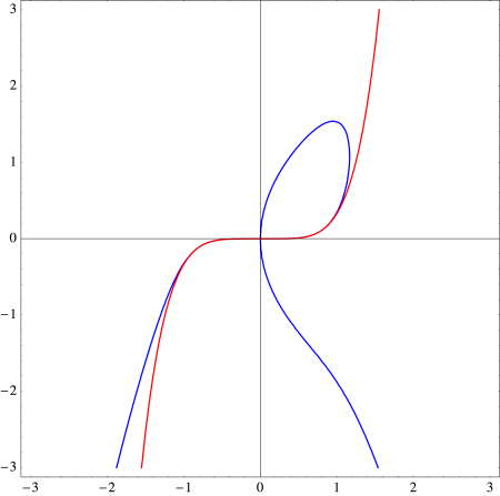

 which results in
 here. But if we move the
  to the other side and factor, we get
 to obtain
 And sure enough, the line
  does the trick:
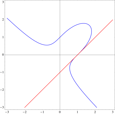


 This results in
 is even, since there is always a root at
  in this case. Here, we make the substitution
  move the
  resulting in
 is a factor of
  so we have

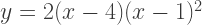
 as well! This is a curious coincidence, for which I have no nice geometrical explanation. The case when
  is illustrated below.
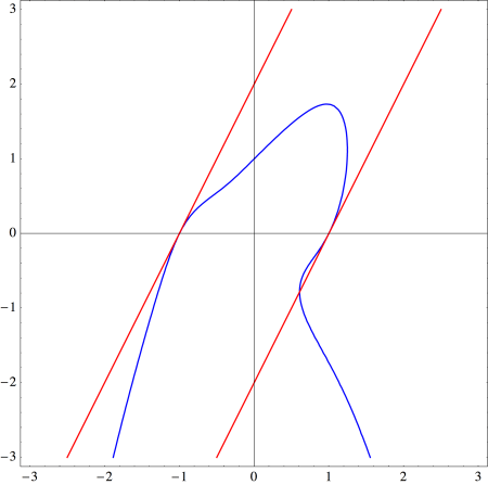


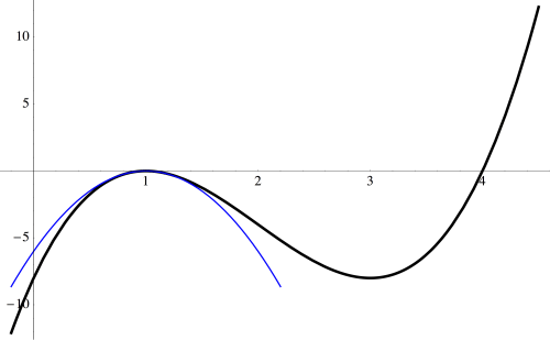
 occurs quadratically.
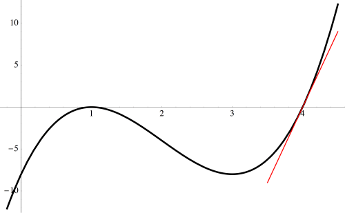
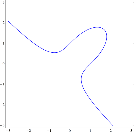
 the graph passes through the x-axis like a line — and we see a linear factor of
  in our polynomial.
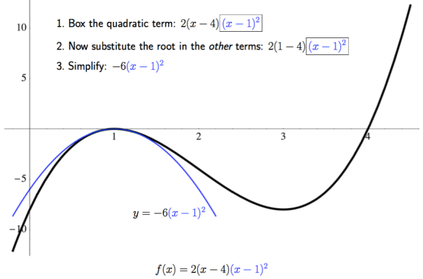
 and substitute the root,
  near the root
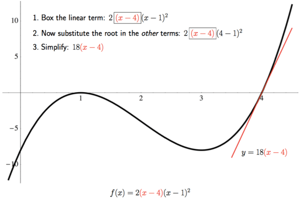
 substitute
  in the remaining terms of the polynomial, and then simplify. Thus, the line
  best describes the behavior of the graph of the polynomial as it passes through the x-axis. Again, note the scale on the axes.
 Begin by sketching the three approximations near the roots of the polynomial. This slide also shows the calculation for the cubic approximation.
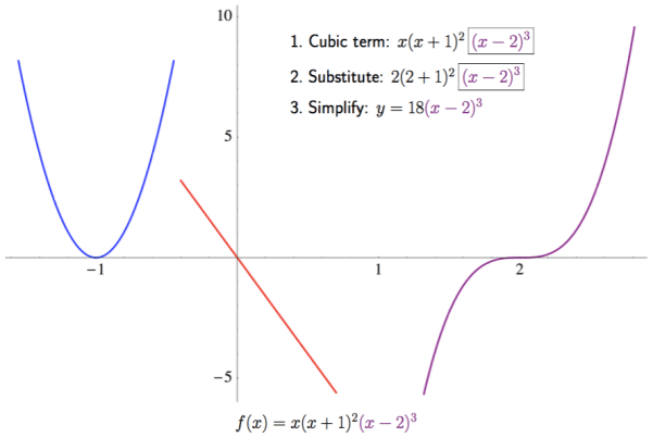

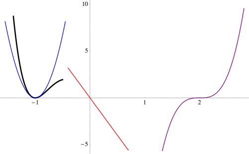
 Of course you’d need to plot a few points to know just where to start and end; this just shows how you would use the approximations near the roots to help you sketch a graph of a polynomial.
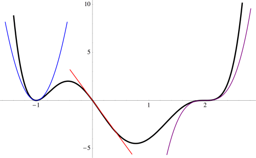
 near the root
  Given what we’ve just been observing, we’d guess that the best approximation near
  would just be
 match at
  derivatives of both of these functions at
  will always be a factor — since at most
  term to completely “disappear.”
 at
at  What about the
  When a derivative of
  is taken, that means one factor of
  we also get
 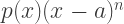 and
and 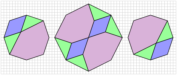
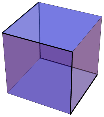
 Imagine a square — a square with side length
  has area
  while a square with side length
  has area
  — which is double the area.
 you need to take a diagonal of a unit square, which rotates the segment by 45° as well as scales it by a factor of
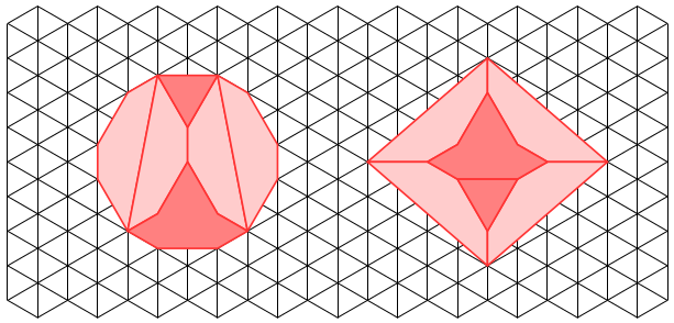
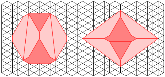
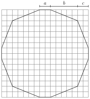
 so that the dodecagon is convex and actually has 12 sides; if
  four pairs of sides are in perfect alignment and the figure becomes an octagon.
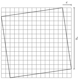
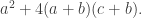 So in order to create a dissection, we must find a solution to the equation
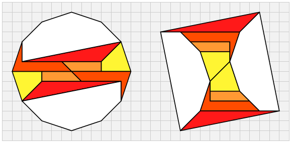
 You get a dissection which looks like this:
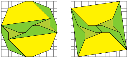


![[OP]\cdot[OP']=1,](https://s0.wp.com/latex.php?latex=%5BOP%5D%5Ccdot%5BOP%27%5D%3D1%2C&bg=ffffff&fg=333333&s=0&c=20201002)
![[AB]](https://s0.wp.com/latex.php?latex=%5BAB%5D&bg=ffffff&fg=333333&s=0&c=20201002) denotes the distance from A to B. Feel free to reread the previous two posts on inversive geometry for a refresher (here are links to the
denotes the distance from A to B. Feel free to reread the previous two posts on inversive geometry for a refresher (here are links to the  Points on a ray drawn from the origin through P will then have coordinates
  where
where  Thus, we just need to find the right
  so that the point
  satisfies the definition of an inverse point.
 and
and  if you substitute
  everywhere you see
  and substitute
  everywhere you see
  From our previous work, we know that the inverse curve must be a circle going through the origin.


 being the origin with coordinates
  ?
? translate to the point
  so that the point

 about the point
 inverted about a series of equally spaced points along the line segment with endpoints
  and
and  This might seem a little arbitrary, but it takes quite a bit of experimentation to find a set of points to invert about in order to create an aesthetically pleasing image.
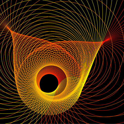

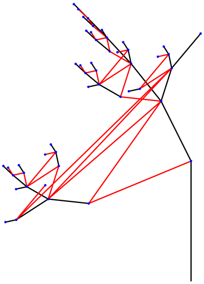
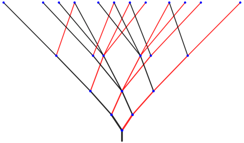
 and that which generate the red branches by
  you will observe behavior like that in the above tree if
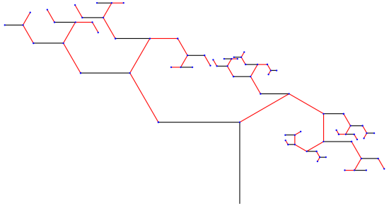
 is a scaled rotation by 60°. This is what produces the spirals of red branches emanating from the nodes of the tree.