October 2016 – Creativity in Mathematics

p-adic Numbers I: When Big is Small

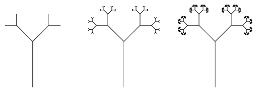
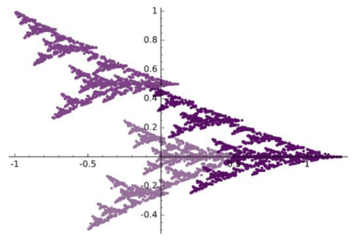
I can’t resist sharing something I just learned about this week. p-adic numbers! I discovered them while exploring angle sequences in creating Koch-like curves, and was immediately fascinated by them. For example, we’ll see that in the field of 5-adic numbers,

$.....444444444 = -1.$

That’s right — the integer with infinitely many 4’s strung together is actually equal to $-1$ ! This seems impossible at first glance, but is actually closely related to

$0.999999999..... = 1$

using decimal numbers.

The subject of p-adic numbers is a broad area in number theory, and we’ll only get a chance to take a small glimpse into it. The simplest examples to look at are related to geometric series. We’ll briefly review them to refresh your memory.

Recall that

$a+ar+ar^2+ar^3+\cdots ar^n+\cdots=\dfrac a{1-r}$

when either $a=0$ or $|r|<1.$

When $r=1,$ for example, the series

$2+2+2+2+2+\cdots$

diverges. To see this, we need to take the sequence of partial sums

$2, 2+2, 2+2+2, 2+2+2+2,\ldots = 2, 4, 6, 8, \ldots,$

which keeps getting larger and larger. By contrast, the series

$1+\dfrac12+\dfrac14+\dfrac18+\cdots\dfrac1{2^n}\cdots$

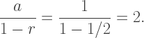
converges because the sequence of partial sums

$1,1+\dfrac12,1+\dfrac12+\dfrac14,1+\dfrac12+\dfrac14+\dfrac18,\ldots=1,\dfrac32,\dfrac74,\dfrac{15}8,\ldots$

keeps getting closer and closer to 2. Of course we can verify the sum with the formula

$\dfrac{a}{1-r}=\dfrac 1{1-1/2}=2.$

The key idea behind discussing convergence is creating a precise mathematical definition of “getting closer and closer to.” This is done using limits (we will not need to go into details here) and the distance function on the real numbers:

$d(x,y)=|y-x|.$

Intuitively, the absolute value of the difference between two numbers is an indication of how close they are.

For a sequence like

$4, 44, 444, 4444, 44,\!444, \ldots,$

which are the partial sums of the geometric series

$4+40+400+4000+40,\!000+\cdots,$

it seems that the terms keep getting further and further apart:

$d(444,4444)=4000,\quad d(4444,44,\!444)=40,\!000,....$

In the field of p-adic numbers, closeness is measured a different way. This might sound strange at first, but let’s consider closeness in plane geometry for a moment.

We are all familiar with the usual distance function in Euclidean geometry:

$d((x_1,y_1),(x_2,y_2))=\sqrt{(x_2-x_1)^2+(y_2-y_1)^2}.$

But maybe you weren’t aware that there are other ways to define distance in the plane — in fact, infinitely many ways — which give rise to non-Euclidean geometries. One of the simplest is

$d_T((x_1,y_1),(x_2,y_2))=|x_2-x_1|+|y_2-y_1|.$

This is often called the taxicab distance, since it describes how far it is from one point to another if you took a taxi on a rectangular grid of streets.

For example, consider going from (0,0) to (3,2) — we’ll use blocks as units — if you could only walk north, south, east, or west. The shortest path might be to go east three blocks, and then north two blocks. Or perhaps north one block, east three blocks, and then north one block again. But the shortest path will always require that you walk five blocks, since you aren’t allowed to walk along a diagonal path. (Note that the shortest path is not always unique in taxicab geometry!)

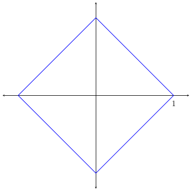
This is a perfectly legitimate geometry, with its own set of properties. For example, the “unit circle” described by the equation

$d_T((x,y),(0,0))=|x|+|y|=1$

is in fact not a circle at all, but a square with vertices at a distance of 1 along the axes!

taxicab

But not any function for distance will work — for example, you’ve got to make sure the triangle inequality is still valid (and it is in taxicab geometry). So while some properties still need to hold, most other properties won’t.

What does this have to do with p-adic numbers? We’re going to look at the positive integers for now, but define close in a very different way. So we can look at some specific examples, let’s take $p=5.$

Here’s the big leap: we say a positive integer is 5-small if there are many factors of 5 in its prime factorization. More specifically, if q is the largest power of 5 which is a factor of n, then the we say that its 5-“size” is

$|n|_5=\dfrac1{5^q}.$

Here are a few more examples, which you should be able to work out for yourself.

$|42|_5=1,\quad |250|_5=\dfrac1{125},\quad |10^{100}|_5=5^{-100}.$

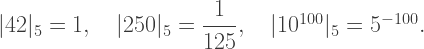
But not everything big is small! For example,

$|10^{100}+1|_5=1,$

since there are no factors of 5 present (which is true for any number ending in a 1).

This may seem odd at first, but when you read more about it, it’s actually amazing. I’ll have to admit that to understand a lot of the amazingness, you’d have to go to grad school in mathematics…. But we’ll get to look at a litte bit of it here.

Before we do, though, there’s another role that 5 plays. We’ve got to write 5-adic numbers in base 5. There’s not room to go into all the details here, but we’ll give a brief review.

Recall that in base 10, we have

$5432_{10}=2+3\times10+4\times10^2+5\times10^3.$

We can only use the digits 0–9.

Now in base 5, we can only use the digits 0–4, and we interpret the digits as follows:

$4302_5=2+0\times5+3\times5^2+4\times5^3=577_{10}.$

We add the same way as we do in base 10, except we carry when we add to more than 5 (and not 10). Thus,

$4_5+3_5=12_5,\quad 34_5+12_5=101_5.$

Subtraction, multiplication, and division are handled similarly.

You won’t need to be an expert in base-5 arithmetic in order to understand how this applies to the equation

$.....444444444 = -1.$

But that will have to wait for the next post on p-adic numbers! We’ll see why this is true, and maybe even talk a little bit about rational p-adic numbers, too….

On Coding III: LISP to Mathematica

The last installment of my coding autobiography was an introduction to LISP. I’d like to continue that discussion today as a segue to talking about Mathematica, because the way I program in Mathematica is heavily influenced by my experience with LISP.

This week I’ll focus on what are typically referred to as aspects of functional programming. Rather than try to explain by using a definition (you can always google it), I’d like to show how I’d perform a simple calculation, like adding the sum of the squares of the first n integers.

Here’s a simple snippet of code which performs this task in Python:

sumsquares

Of course you could embed the square function in the loop, but for more complicated functions, this is not usually done. In any case, I’m using this approach to illustrate a point.

Now in Mathematica, I would write:

mmasumsq

You might think that there’s no way the code could be shrunk that much, but it really is possible. Let’s see why.

We’ll look at the “# * # &” piece first. This is usually called a pure function, and is essentially a function with no name. It’s like defining f(#) to be # * #, and then invoking f. But with the “#” as the argument to the function, this syntax allows you to avoid naming the function altogether.

Why might you want to do this? One reason is it makes your code less cluttered if you need to define a relatively simple function and use it just once. I actually use pure functions a lot. Once you start thinking about programming with them in mind, it really does help streamline your code. You find you can’t live without them, and when you use a language which doesn’t allow them, you really miss ’em….

What about the “/@”? This is a map, and is the alternative to iteration in LISP. What it says is this: “Here is a function, and here is a list of arguments. Apply the function to each of the elements of the list in order, and collect the results in a new list.” So

# * # & /@ {1,2,3}

would return the list {1,4,9}.

In languages like LISP and Mathematica, the use of maps is built in to the heart of the compilers, so that maps are often much faster than iterating. In fact, to add the squares of the first 1,000,000 integers, it’s about 40 times faster in Mathematica to use a map than to use a loop. I can remember a time I was using iteration to create fractals in Mathematica, and it was taking around 10 minutes to generate each one. For fun, I thought I’d try using maps, and the run time decreased to less than 30 seconds! It can really make a difference.

There are more complicated ways to use maps which involve functions of more than one argument, and assembling arguments from lists in different ways. But the example above illustrates the basic idea.

Of course the use of Range[n] is familiar to Python users, and returns a list of the first n integers, starting with 1 — unlike Python, though, where the list begins at 0. Personally, for much of what I do, I much prefer the list to begin at 1. I tend to use “i+1” a lot when I use range(n) in Python.

Finally, what about the “@@”? This is like the apply function in LISP I described in my last post. Essentially, it means take this function, Plus, and apply it to this list of numbers, in this case the squares of the first n integers. It saves having to write a loop which successively adds each next number to a running total. As an example, it is easy to write a factorial function in Mathematica:

Times @@ Range[n].

So that’s how to sum the squares of the first n integers in just a half line of code! Now these ideas can all be implemented in LISP and Python as well, and other languages which include more functional apsects. But for simplicity of syntax, I prefer Mathematica over the others.

The point of using Mathematica code for this example is to show how my style of programming in Mathematica is really very LISP-like. In fact, I’ve had the experience of showing code like this to some Mathematica programmers, and needing to explain it just like I did for you here. This is because if you learned a language like PASCAL, C, or some other procedural language, you can code in Mathematica exactly the same way, without ever knowing anything about the functional aspects.

Back to a little history…. I did all my undergraduate and graduate work at Carnegie Mellon, and beginning with my sophomore year as an undergrad, was working a lot with LISP while teaching with the PGSS. Mathematica was first released during my second year of graduate school, and CMU being the type of school it was, Mathematica was readily available. I can recall working with it on a NeXT computer. (Google it!)

So I was introduced to Mathematica while I was heavily into LISP — and found that I was really excited that I could do so many LISP-like things in Mathematica! More about Mathematica in my next installment of On Coding….

Frankly, I rarely use LISP now. I do recall creating an address book in LISP — having a list of addresses and phone numbers in a long list, and using LISP to output LaTeX code which I could then run and print out a nicely formatted array of addresses. But other than that, little else comes to mind.

But although I don’t use the language itself, learning to program in LISP has definitely influenced my programming style more than any other coding experience. I always encourage my students to study it as a result — although functional programming ideas are now incorporated into many other languages, it’s easy to learn the concepts elsewhere.

For me, I’ll always have a special place in my hacker heart for all those idiotic stupid parentheses….

Digital Art IV: End of Week 8

The last two weeks were focused on a study of polyhedra. While not strictly a digital art topic, I thought it important for students to develop a basic three-dimensional vocabulary in the event they wanted to do further study in computer graphics.

imag4281

We began with the Platonic solids, naturally, looking at enumerating them geometrically and algebraically. The algebraic enumeration involved solving the usual

$\dfrac1p+\dfrac1q=\dfrac12+\dfrac1E.$

This proved challenging, especially when I gave some additional, similar Diophantine equations for homework. We also took time to build a dodecahedron and an icosahedron. This occupied us on Day 17, Day 18, and part of Day 19.

Since the first half of the semester was nearing its end, it was time to begin thinking about Final Projects. So I took the rest of Day 19 to help students individually choose a topic, and assigned the Project Proposal over the weekend.

We had a brief discussion of graph theory on Day 20, which involved looking at the adjacency graphs of the vertices of the Platonic solids, such as the one for the dodecahedron.

graphdodeca

I introduced much of the basic vocabulary, using the chapter I wrote in my polyhedra textbook as a guide. Of course there is only so much progress to be made during a single class, but I did want to indicate how two apparently different areas in mathematics are related.

The homework involved untangling adjacency graphs, such as the one below.

graphprism

This is just a triangular prism, although drawn a little unconventionally. This assignment again proved more difficult than I thought, even with Euler’s formula to help in calculating the number of faces. So we spent extra time on Day 21 going over the homework, followed by a very brief discussion of duality. And as students were having difficulty narrowing their focus for their project proposals, I spend the rest of Day 21 talking individually with them as they started building a few rhombic dodecahedra.

Over half of Day 22 was taken up by a quiz on their homework; I didn’t want there to be much time pressure. The last part of this class was spent creating an in-class sculpture with rhombic dodecahedra. I chose this dual model for them to build as it is space-filling.

I was surprised at how much they really got into it! I do hope we have time for a similar project at the end of the semester. We were in a bit of a rush for time, but still managed to create something intriguing.

imag4318

Last time I mentioned I assigned a short response paper getting feedback from the students about how the course was going so far, and I said I’d share some of their comments. All (anonymous) quotes are from student papers.

I really like how hands-on the course is, and how there is a good balance between lecture and lab time.

This was a common opinion — and validates a major feature of the course design. I am glad students appreciate it! Another student made a similar remark about the lab time.

I enjoy the lab assignments that we get because I like the designs I create. It allows us to put to practice what we have learned with each lesson.

I specifically asked about how students’ attitudes about mathematics changed. I got some encouraging responses.

I was used to thinking of math as just something I had to do, that would probably be useful later in life, but wouldn’t really pertain to whatever I wanted to do with art. I’ve realized that I would actually really like to use this kind of math in my art in the future, because I never realized what kind of things I could make with this medium.

As someone who wasn’t the best at geometry in high school (I’m more of an algebra person), I think this class has given me a practical use for all the things I learned in high school that I found difficult to grasp or uninteresting.

I was pleased to read responses like this, since again, this reflects an overarching purpose of the course — see how mathematics can actually be used in practice. One student even went so far as to say,

I would also like to mention something, though this might not be considered significant, I never thought I would have to use matrices ever again in my life.

A few students remarked on using mathematics in the creative process.

At first, I was a little unsure of the role that mathematics took in graphic design, but as soon as we started playing with Sage, I noticed that it affects almost every aspect brought forth in the image.

Making “rules” for you art was something very different for me…..combining the left brain and the right brain creates incredible pieces of work….

Some students made more specific comments. One student liked the presentations the best.

Looking through the different papers in the Bridges archive and hearing everyone’s presentations really made me realize the extent that mathematics is related to so many other topics.

In addition, I asked for specific suggestions for improvement. By far the most common remark was that students want to learn more about how the Python code in Sage works. I was really encouraged when I read those comments! We will start to learn Processing in a few weeks, and I’ll make sure we discuss the code in more detail.

One student really liked the discussion board I set up for a few of the assignments — it is not difficult to create discussion boards for future assignments, so we’ll try that again. Another remarked that it would be good to learn about the printing process — and I certainly agree! But as I remarked in previous posts, I thought the logistics of this challenging endeavor would be too difficult to implement. It is certainly a future goal.

But overall, I was very glad to read how students were enjoying the course — and also pleased about their suggestions for improvement. So I’ll work hard at making the second half of the course even better than the first!

Koch Curves and Canopies

Time for another “math in the moment” post! There have been a few interesting developments just this past week, so I thought I’d share them with you.

The first revolves around the Koch curve. I’ve talked a lot about the algorithm used to generate the Koch curve when the angles are changed — but this is the first time I’ve experimented with three different angles. For example, the recursive procedure

F +45 F +180 F +315 F

generates the following spiral:

spiral8

Looks simple, right? Just 16 line segments. But here’s the unexpected part — it takes 21,846 iterations to make! That’s right — the horizontal segment in the upper left is the 21,846th segment to be drawn.

Why might this be? Partly because of the fact that one angle is 180, and also the fact that 45 + 415 = 360. In other words, you are often just turning around and retracing your steps. These arms are retraced multiple times, not just once or twice like in previous explorations.

I found this family of spirals by having Mathematica generate random angles and using the algorithm to draw the curves. Without going into too many details, the “obvious” way to generalize the equation I came up with before didn’t work, so I resorted to trial and error — which is easy to do when the computer does all the work!

Notice the pattern in the angles: 45 (1/8 of a circle), 180 (1/2 of a circle), and 315 (7/8 of a circle). Moving up to tenths, we get angles of 36 (1/10 of a circle), 180 (1/2 of a circle), and 324 (9/10 of a circle), which produce the image below.

Notice there are only five arms this time (not 10). And it only takes 342 segments to draw! There’s an alternating pattern here. Moving up to twelfths gives 12 arms, and takes a staggering 5,592,406 segments to draw. Yes, it really does take almost 6,000,000 iterations to draw the 24th and last segment!

With the help of Mathematica, though, I did find explicit formulas to calculate exactly how many iterations it will take to draw each type of image, depending on whether there are an even number of arms, or an odd number. Now the hard part — prove mathematically why the formulas work! That’s the next step.

I hope this “simple” example illustrates how much more challenging working with three different angles will be. I think working out the proof in these cases will give me more insight into how the algorithm with three angles works in general, and might help me derive an equation analogous to the case when the first and third angles are the same.

The second development is part of an ongoing project with Nick to write a paper for the Bridges 2017 conference in Waterloo. The project revolves around fractal trees generated by L-systems. (We won’t be discussing L-systems in general, but I mention them because the Wikipedia had a decent article on L-systems.)

trees1

Consider the examples above. You first need to specify an angle, a, and a ratio, r. In this example, a is 45 degrees, and r is 0.5. Start off by drawing a segment of some arbitrary length (in this case the trunk of a tree). Then turn left by the angle a, and recurse using the length scaled by a factor of r. When this is done, do the same recursion after turning right by the angle a.

On the left, you should see three different sized lengths, each half the size of the one before. You should also be able to easily see the branching to the left and right by 45 degrees, and how this is done at each level.

In the middle, there are six levels, with the smallest branches only 1/32 the length of the tree trunk. Can you guess how many levels on the right? There are twelve, actually. At some point, the resolution of the screen is such that recursing to deeper levels doesn’t actually make the fractal look any different.

What Nick is interested in is the following question. Given an angle a, what is the ratio r such that all the branches of the tree just touch? In the example below with a being 45 degrees, the leaves are just touching — increasing the ratio r would make them start to overlap.

trees2

What is r? It turns out that there’s quite a bit of trigonometry involved to find the precise r given an angle a, but it’s not really necessary to go into all those details. It’s just enough to know that Nick was able to work it out.

But what Nick is really interested in is just the canopies of these trees — in other words, just the outermost leaves, without the trunk or any of the branches.

canopy1

Right now, he’s experimenting with creating movies which show the canopies changing as the angle changes — sometimes the ratio is fixed, other times it’s changing, too.

Two observations are worth making. First, this was a real team effort! Nick had done the programming and set up quite a bit of the math, and with the aid of Mathematica, I was able to help verify conjectures and get the expressions into a useable form. We each had our own expertise, and so were each able to contribute in our own way to solving the problem.

Second, Nick is using mathematics to aid in the design process. My first attempts to create symmetric curves using the algorithm for the Koch snowflake were fairly random. But now that I’ve worked out the mathematics of what’s going on, I can design images with various interesting properties.

Likewise, Nick has in mind a very particular animation for his movies — using the just-touching canopies — and is using mathematics in a significant way to facilitate the design process. Sure, you can let the computer crunch numbers until you get a good enough approximation — but the formula we derived gives the exact ratio needed for a given angle. This is truly mathematical art.

I’ll keep you updated as more progress is made on these projects. I’ll end with my favorite image of the week. The idea came from Nick, but I added my own spin. It’s actually canopies from many different trees, all superimposed on each other. Enjoy!

canopy2

Digital Art III: End of Week 6

Recall that at the end of Week 4, we had just begun a lab on affine transformations and iterated function systems. At the beginning of Week 5 (Day 11), students were supposed to finish the exercise they began on Friday, and try another. This was the new prompt: Create a fractal using two affine transformations. For the first, rotate by 60 degrees, then scale the x by 0.6 and the y by 0.5. For the second transformation, rotate 60 degrees clockwise, scale the x by 0.5 and the y by 0.6, and then move to the right 1. I provided a link to the fractal which should be produced, shown below.

$d11fractal$

Again, this proved to be a challenge! The reason is that the computer is somewhat unforgiving. To produce the image above, every calculation has to be correct. Here were some common issues:

There was difficulty interpreting the statements as geometric transformations. In particular, getting the order of the matrix multiplication correct, and interpreting a clockwise rotation as a rotation by -60 degrees.
Performing the matrix multiplication correctly. Some students were using online calculators, and some had trouble with converting degrees to radians.
Translating the results into Python code; the affine transformations needed to be converted to the form $(ax+cy+e, bx+dy+f).$

I also gave them an exercise to reproduce one of the fractals they needed to analyze for homework the previous week.

This occupied us for all of Week 5, since I also wanted to give them time to work on their upcoming assignment.

Week 6 was our first Presentation Week. Since we’d only need two days for the presentations given the class size, I spent the first day of the week giving my Bridges talk on producing Koch-like fractal images.

The class was interested to learn more about this algorithm, and I had hoped to spend a week devoted to the topic. But because of the Processing work we’ll be doing later — animation of fractals using iterated function systems — I didn’t want to rush through the preliminary work on affine transformations and IFS. Any misunderstandings now would surely be problematic later.

The presentations were to be on papers from the Bridges archives. All papers since the Bridges conferences began (which was in 1998) are archived online. The assignment was simple: find a paper in the archive that’s at least four pages long, and give a five-minute presentation on it to the class. I did create a discussion board where they posted the title/author of their selections so there wouldn’t be any duplicate presentations.

These presentations went very well. Most students’ presentations were close to ten minutes long, and the enthusiasm for their presentations was quite evident. I must admit that I learned a lot, too — I had not read most of the papers they selected.

I had students do simple peer evaluations, and included the item “I would like to learn more about this topic after hearing the presentation.” They selected a number from 1–5, with 5 meaning “most interested.” The overall average score was about 3.9 — meaning the papers piqued their curiosity. In addition, I wanted to get additional ideas about what to include in the few days I set aside for special topics at the end of the semester, or what new ideas to incorporate into next semester’s class.

The most popular paper (4.75 average) was On Generating Dot Paintings in the Style of Howard Arkley, which Madison said reminded her of some of the textures we created during a few of our lab sessions. The next highest average was 4.25, so this was the clear favorite. I hope we’ll have time to explore it further later on.

And that took us to the end of Week 6! I had hoped to have some time in the lab to have students find interesting polyhedra nets they’d like to build, since the next two weeks will be devoted to polyhedra. No, it’s not really a digital art topic — but it is an area of expertise. I wanted students to have some exposure to three-dimensional geometry since if they continue to study computer graphics, they will certainly move from two into three dimensions.

Now it’s time to look at some student work! I’ll focus on one fractal from the assignment on iterated functions systems. Here is the prompt: Create a morphed Sierpinski triangle, based on the code in the Sage worksheet. The idea is to have your fractal look like it was derived from a Sierpinski triangle, but just barely. Someone looking at it should wonder about it, and maybe after 30 seconds or so, say “Hey, that looks like a Sierpinski triangle!”

One student created the following image, and wrote:

I think this fractal looks like many sets of pine trees, and I like the way that it shears out. I made the whole thing the same color (gray) to make the fact that it was derived from the Sierpinski triangle less obvious.

af2

Julia creating the following fractal image, and remarked that at one point, she went “too far” and had to backtrack a bit.

jn3

Safina went a different direction, and created this.

sm4

She wrote,

The stretch and rotation reminds me of a tree, more specifically a Christmas tree….I wanted to emulate a sort of Christmas feel because I was listening to Christmas music.

So motivation can come from anywhere! I’ll post more of their images on my Twitter feed, @cre8math.

Again, you can see how my students are really embracing the course and being very creative with the assignments. I’m looking forward to seeing more of their work.

I just assigned a brief response paper asking students how they felt about the course so far, and how it has changed their ideas about art, mathematics, and computer science. I’ll report on their comments in my next summary in two weeks. Stay tuned!