May 2016 – Creativity in Mathematics

Making Movies with Processing IV

Last week, we saw how using linear interpolation allowed us to create animations of fractals. This week, we’ll explore how to create another special effect by using linear interpolation in a different way. We’ll build on last week’s example, so you might want to take a minute to review it if you’ve forgotten the details.

Let’s suppose that in addition to morphing the Sierpinski triangle, we want to slowly rotate it as well. So we insert a rotate command before plotting the points of the Sierpinski triangle, as shown here:

CodeSnippet1

First, it’s important to note that the rotate command takes angles in radian measure, not degrees. Recall from your trigonometry classes that

$360^\circ=2\pi{\rm \ radians.}$

But different from your trigonometry classes is that the rotation is in a clockwise direction. When you studied the unit circle, angles moved counter-clockwise around the origin as they increased in measure. This is not a really complicated difference, but it illustrates again how not every platform is the same. I googled “rotating in processing” to understand more, and I found what I needed right away.

Let’s recall that p is a parameter which is 0 at the beginning of the animation, and 1 at the end. So when p = 0, there is a rotation of 0 radians (that is, no rotation), and when p = 1, there is a rotation of $2\pi$ radians, or one complete revolution. And because we’re using linear interpolation, the rotation changes gradually and linearly as the parameter p varies from 0 to 1.

Let’s see what effect adding this line has. (Note: Watch the movie until the end. You’ll see some blank space in the middle — we’ll explain that later!)

What just happened? Most platforms which have a rotate command assume that the rotation is about the origin, (0,0). We learned in the first post that the origin in Processing is in the upper left corner of the screen. If you watch that last video again, you can clearly see that the Sierpinksi triangle does in fact rotate about the upper left corner of the screen in a clockwise direction.

Of course this isn’t what we want — since most of the time the fractals are out of the view screen! So we should pick a different point to rotate around. You can pick any point you like, but I though it looked good to rotate about the midpoint of the hypotenuse of the Sierpinski triangles. When I did this, I produced the following video.

So how did I do this? It’s not too complicated, but let’s take it one step at a time. We’ve got to remember that before scaling, the fractal fit inside a triangle with vertices (0,0), (0,2), and (2,0). I wanted to make it 450 pixels wide, so I scaled by a factor of 225.

This means that the scaled Sierpinski triangle fits inside a right triangle with vertices (0, 0), (0, 450), and (450, 0). Using the usual formula, we see that the midpoint of the hypotenuse of this triangle has coordinates

$\dfrac12\left((0,450)+(450,0)\right)=(225,225).$

To make (225, 225) the new “origin,” we can just subtract 225 from the x– and y-coordinates of our points, like this:

CodeSnippet2

Remember that the positive y-axis points down in Processing, which is why we use an expression like 225 – y rather than y – 225. This produces the following video.

This isn’t quite what we want yet, but you’ll notice what’s happening. The midpoint of the hypotenuse is now always at the upper left corner. As the triangle rotates, most of it is outside the view screen. But that’s not hard to fix.

All we have to do now is move the midpoint of the hypotenuse to the center of the screen. We can easily do this using the translate function. So here is the complete version of the sierpinski function, incorporating the translate function as well:

CodeSnippet3

So let’s briefly recap what we’ve learned. Rotating an image is not difficult as long as you remember that the rotate function rotates about the point (0,0). So first, we needed to decided what point in user space we wanted to rotate about – and we chose (225, 225) so the fractals would rotate around the midpoint of the hypotenuse of the enclosing right triangle. This is indicated in how the x– and y-coordinates are changed in the point function.

Next, we needed to decided what point in screen space we wanted to rotate around. The center of the screen seemed a natural choice, so we used (384, 312). This is indicated in the arguments to the translate function.

And finally, we decided to have the triangles undergo one complete revolution, so that p = 0 corresponded to no rotation at all, and p = 1 corresponded to one complete revolution. We accomplished this using linear interpolation, which was incorporated into the rotate function.

But most importantly — we made these changes in the correct order. If you played around and switched the lines containing the translate and rotate functions, you’d get a different result.

It is worth remarking that it is possible to use the rotate function first. But then the translate function would be much more complicated, since you would have to take into account where the point (384, 312) moved to. And you’d have to review your trigonometry. Here’s what the two lines would need to look like:

CodeSnippet4

As you can see, there is a lot more involved here! So when you’re thinking about designing algorithms to produce special effects, it’s worth thinking about the order in which you perform various tasks. Often there is a way that is easier than all the others — but you don’t always hit upon it the first time you try. That’s part of the adventure!

Next week we’ll look a few more special effects you can incorporate into your movies. Then we’ll look at actual movies made by students in my linear algebra class. They’re really great!

Making Movies with Processing III

This week, we begin a discussion of creating movies consisting of animated fractals. Last week’s post about the dot changing colors was at a beginning level as far as Processing goes. This week’s post will be a little more involved, but will assume a knowledge of Iterated Function Systems. I talked about IFS on Day034, Day035, and Day036. Feel free to look back for a refresher….

Today, we’ll see how to create the following movie. You’ll notice that both the beginning and final Sierpinski triangles are fractals discussed on Day034.

As a reminder, these are the three transformations which produce the initial Sierpinksi triangle:

$F_1\left(\begin{matrix}x\\y\end{matrix}\right)=\left[\begin{matrix}0.5&0\\0&0.5\end{matrix}\right] \left(\begin{matrix}x\\y\end{matrix}\right),$

$F_2\left(\begin{matrix}x\\y\end{matrix}\right)=\left[\begin{matrix}0.5&0\\0&0.5\end{matrix}\right] \left(\begin{matrix}x\\y\end{matrix}\right)+\left(\begin{matrix}1\\0\end{matrix}\right),$

$F_3\left(\begin{matrix}x\\y\end{matrix}\right)=\left[\begin{matrix}0.5&0\\0&0.5\end{matrix}\right] \left(\begin{matrix}x\\y\end{matrix}\right)+\left(\begin{matrix}0\\1\end{matrix}\right).$

Also, recall that to get the modified Sierpinski triangle at the end of the video, all we did was change the first transformation to

$F_1\left(\begin{matrix}x\\y\end{matrix}\right)=\left[\begin{matrix}0.25&0\\0&0.5\end{matrix}\right] \left(\begin{matrix}x\\y\end{matrix}\right).$

We’ll how to use linear interpolation to create the animation. But first, let’s look at the Python code for creating a fractal using an iterated function system.

ifscode

The parameter p is for the linear interpolation (which we’ll discuss later), and n is the number of points to plot. First, import the library for generating random integers — since each transformation will be weighted equally, it’s simpler just to choose a random integer from 1, 2, and 3. The variable points keeps track of all the points, while last keeps track of the most recently plotted point. Recall from earlier posts that you only need the last point in order to get the next one.

Next, the for loop just creates new points, one at a time, and appends them to points. Once an affine transformation is randomly chosen by selecting a randint in the range from 1 to 3, it is applied to the last point generated. For the purpose of writing Python code, it’s easier to use the notation

$F_2\left(\begin{matrix}x\\y\end{matrix}\right)=\left(\begin{matrix}0.5 \ast x+1\\0.5\ast y\end{matrix}\right)$

rather than matrix notation. In order to use vector and matrix notation, you’d need to indicate that (1,2) is a vector by writing

v = vector(1,2),

and similarly for matrices. Since we’re doing some fairly simple calculations, just writing out the individual terms of the result is easier and requires less code.

Once the points are all created, it’s time to plot them. You’ll recognize the background, stroke, and strokeWeight functions from last week. Nothing fancy here, since we’re focusing on algorithms today. Just a black background and small orange dots.

The last line plots the points, and is an example of what is called list comprehension in Python. First, note that the iterated function system would create a fractal which would fit inside a triangle with vertices (0,2), (0,0), and (2,0). So we need to suitably scale the fractal — in this case by a factor of 225 so it will be large enough to see. Remember that units are in pixels in Processing.

Then we need to compensate for Processing’s coordinate system. You’ll notice a similarity to what we did a few weeks ago.

What the last line does is essentially this: for every point x in the list points, adjust the coordinates for screen space, and then plot x with the point function. List comprehension is convenient because you don’t have to make a loop or other iterative construct — it’s done automatically for you.

Of course that doesn’t mean you never need a for loop. It wouldn’t be easy to replace the for loop above with a list comprehension as each new point depends on the previous one. But for plotting a bunch of points, for example, it doesn’t matter which one you plot first.

Now for the linear interpolation! We want the first frame to be the usual Sierpinski triangle, and the last frame to be our modified triangle. The only difference is that one of the constants in the first function changes from 0.5 to 0.25.

This is perfect for using linear interpolation. We’d like our parameter p to be 0.5 when p = 0, and 0.25 when p = 1. So we just need to create a linear function of p which passes through the points (0, 0.5) and (1, 0.25). This isn’t hard to do; you should easily be able to get

$0.5 - 0.25 \ast p.$

The effect of using the parameter p in this way is to create a series of fractals, each one slightly different from the one before. Since we’re taking 360 steps to vary from 0.5 to 0.25, there is very little difference from one fractal to the next, and so when strung together, the fractals make a convincing animation.

I should point out the dots look like they’re “dancing” because each time a fractal image is made, a different series of random affine transformations is chosen. So while the points in each successive fractal will be close to each other, most of them will actually be different.

For completeness, here is the code which comes before the sierpinski function is defined.

ifscodesetup2

It should look pretty familiar from last week. Similar setup, creating the parameter p, writing out the frames, etc. You’ll find this a general type of setup which you can use over and over again.

So that’s all there is to it! Now that you’ve got a basic grasp of Processing’s screen space and a few different ways to use linear interpolation, you can start making movies on your own.

Of course there are lots of cool effects you can add by using linear interpolation in more creative ways. We’ll start to take a look at some of those next week!

Making Movies with Processing II

Last week we learned a little about the history of Processing, as well as what the coordinate system is like in Processing (and many other graphics applications as well). Today I’d like to discuss an idea which I find very helpful in making movies — linear interpolation. We’ll only have time for one simple example today, but we’ll go through that example very thoroughly.

So here’s the movie we’ll explore today. Not glamorous, but it’s a start.

You’ll notice what’s happening — the dot slowly turns from magenta to black, while the background does the opposite. Let’s look at the dot first. In Processing, RGB values go from 0 to 255. Magenta is (255, 0, 255) in RGB, and black is (0, 0, 0). We want the dot to go smoothly from magenta to black.

The way I like to do this is to introduce a parameter p. I think of p = 0 as my starting point, and p = 1 as my ending point. In this example, p = 0 corresponds to magenta, and p = 1 corresponds to black. As p varies from 0 to 1, we want the dot to go from magenta go black.

This is where linear interpolation comes in. For any start and end values, the expression

(1 – p) * start + p * end

will vary continuously from the start value to the end value as p goes from 0 to 1. It should be clear that when p = 0, you get the start value, and when p = 1, you get the end value. Any value of p in between 0 and 1 will be in between the start and end values — closer to the start value when p is near 0, and closer to the end value when p is near 1.

Because this expression is linear in p — no quadratic terms, no square roots, no sines or cosines — we say that this expression gives a linear interpolation between the start and end values.

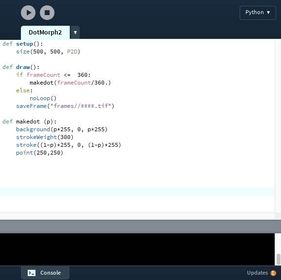
Let’s see how this works in Processing. Here’s a screen shot of the code that produced the video shown above.

screenshot2

The basic functions for making a simple movie are setup and draw. The setup function is executed once before the movie starts. Then the draw function is called repeatedly — each time the draw function is called, a new frame of the movie is created.

In a typical program, if you wanted to repeat something over and over, you’d need to make a loop. But in Processing — since its purpose is to create frames for movies — this is built in to how the application works. No need to do it yourself.

So in Processing, the variable frameCount automatically keeps track of which frame you’re creating. And it is automatically incremented each time the draw function executes. You’ll find that this is a very nice feature! This way, you don’t have to keep track of frames yourself.

Note the size declaration in the setup function. Last week, I mentioned that you’ve got to set the size of your coordinate system when you start your movie. The “P2D” means you’re creating a two-dimensional image. You can make 3D objects in processing, but we won’t look at that today.

Typical applications which make movies (like PhotoShop, or the Movie Maker found in Processing’s “Tools” menu) use about 30 frames per second. So 360 frames (as above) will be a 12-second movie. Enough to see the dot and background change colors.

The if/else clause determines the frames produced. Note that when frameCount gets larger than 360, you skip to the “else” clause, which is “noLoop()”. This essentially stops Processing from creating new frames. The saveFrame command saves the individual frames to whatever directory you specify; if you forget the else clause, Processing will just keep generating more and more .tiff files and clutter up your directory.

So the if/else clause basically tells Processing this: make 360 frames, one at a time, and save then in a directory called “frames.” Once all 360 frames are made, it’s time to stop.

The makedot function is what actually creates the frame. Now we’re getting to the linear interpolation! The frameCount/360. is what creates the value of p. When frameCount is 1, the value of p is 1/360 (close enough to 0 for the purposes of our movie), and when frameCount is 360, the value of p is 1. As the value of frameCount increases, p increases from about 0 to 1.

It’s important to use a decimal point after the number 360. If you don’t, Python will use integer division, and you’ll get 0 every time until frameCount reaches 360, and only then will you get 1. (I learned this one the hard way…took a few minutes to figure out what went wrong.)

So let’s go through the makedot function line by line. First, we set the background color. Note that when p is 0, the color is (0, 0, 0) — black. As p moves closer to 1, the black turns to magenta. It is also important to note that when you call the background function, the entire screen is set to the color you specify. Processing will write over anything else that was previously displayed. So be careful where you put this command!

Next, the width of lines/points drawn is set with strokeWeight. Remember that the units are pixels — so the width of the dot is 300 pixels on a screen 500 pixels wide. Pretty big dot.

The stroke command sets the color of lines/points on the screen. Notice the (1 – p) here — we want to begin with magenta (when p = 0), and end with black (when p = 1). So we go the “opposite” direction from the background.

Maybe you noticed that at one point, the dot looked like it “disappeared.” Not really — note that when p = 1/2, then 1 – p = 1/2 as well! At this time, the dot and background are exactly the same color. That’s why it looked like the dot vanished.

And last but not least — the dot. Remembering the coordinate system, the dot is centered on the screen at (250, 250).

That’s it. Not a long program, but all the essentials are there. Now you’ve got a basic idea of how simple movies can me made. The next post will build on this week’s and look at some more examples of linear interpolation. Stay tuned!

Making Movies with Processing I

If you’ve been following my Twitter (@cre8math), you’ll have noticed I posted quite a few videos last fall. At the time I was writing a lot about creating fractal images, and I really wanted to learn how to make animations using these images. I had heard about Processing from a lot of friends, and decided that it was time to dive in! Here is one of earlier movies, but still one of my favorites.

Processing has been around since 2001. From the very beginning, Processing was used in the classroom as a tool to allow students to quickly create graphical images and movies. It is now used widely by educators, artist, designers, architects, and researchers. Many companies use Processing for data visualization. Click on the link to read more!

One of the great things about Processing is that it’s open source — a specific intention of the developers. Now, there’s even a Processing Foundation. Its purpose is to “promote software literacy within the visual arts, and visual literacy within technology-related fields — and to make these fields accessible to diverse communities.” The idea is to provide everyone access to software you can use to create a wide range of visual media. Not just those who can afford it.

I support open-source initiatives as well. Most of the digital art I’ve talked about on my blog was written in Mathematica, a powerful programming language, but expensive to buy. I rewrote all the algorithms you’ve seen on the Sage worksheets in Python because I wanted them to be available to anyone who has access to the internet. Not just those who can afford pricey software….

Now there won’t be time to go into everything about Processing — that’s what the internet is for. I often google phrases like “How do you change the background color in Processing?”, and usually get the information I need pretty quickly.

What I want to focus on today is the coordinate system used in Processing. If you’re new to computer graphics, it might be a little unfamiliar — the coordinate system is based on pixels. For example, the screen on my Mac is 1440 x 900 pixels. But the origin (0, 0) is in the upper left corner of the screen, so that the lower right corner has coordinates (1440, 900). In other words, while the positive x-axis is still to the right, the positive y-axis is now pointing down. This is sometimes called a screen coordinate system, or screen space.

This convention has an interesting history. Older television screens used cathode ray tubes, and literally updated the screen by refreshing one line at a time, from top to bottom and from left to right. After updating the pixel at the lower right, refreshing began again at the upper left. This process occurred several times each second to give the illusion of continuous motion. Because the refresh was done from top to bottom, the y-coordinates increased from top to bottom as well.

Such a coordinate system is not unusual. The PostScript programming language (which I told you about two weeks ago) has a coordinate system based on points. The definition of a point has changed over time, but PostScript uses a coordinate system where there are 72 points per inch, and the lower left corner has coordinates (0,0).

PostScript is used for printing physical documents. Because copier paper typically has dimensions 8.5″ x 11″ in the United States, the upper right corner of your document would have coordinates (612, 792).

In Processing, you need to specify the size of the screen you want for your movie. In the example above, I chose 768 x 768 pixels. This may sound like a strange number, but a commonly used screen size is 1024 x 768. Because of what my image looked like, though, I wanted the screen to be square so there wouldn’t be extra space on the left and right.

Now the objects you see in the movie have rotational symmetry. So it would make sense for the origin (0,0) to be at the center of the movie screen, not the upper left corner. A convenient coordinate system for these objects might have the upper left corner be (-1, 1), and the lower right corner be (1, -1), just like the usual Cartesian coordinate system. This system of coordinates is sometimes called local space or user space. In other words, it’s the space the user is thinking in when designing various images.

So now the issue is converting from user space to screen space. This isn’t difficult, so we’ll just work through this example to see how it’s done. All you need to remember is how to find the equation of a line.

Why a line? Let’s look at x-coordinates first. In user space, x-coordinates range from -1 to 1. In screen space, they range from 0 to 768. If you went 1/4 of the way from -1 to 1 in user space — which would put you at -0.5 — then you’d expect the corresponding point in screen space to be 1/4 of the way from 0 to 768, which would be 192. You’d expect this for any ratio, not just 1/4. This is precisely what it means for the transformation of coordinates from user space to screen space to be linear.

Since -1 in user space corresponds to 0 in screen space, and 1 corresponds to 768, all we need to do is find the equation of the line between the points (-1,0) and (1,768). In Cartesian coordinates, this would be $y=384(x+1).$ Or we might alternatively say

$x_{\rm screen} = 384(x_{\rm user}+1).$

Once we know how to do this for the x-coordinates, we can proceed the same way for the y-coordinates. You should be able to figure out that

$y_{\rm screen} = 384(1-y_{\rm user}).$

Note that the minus sign in front of $y_{\rm user}$ is a result of the fact that the positive y direction is pointing down.

This is a very general idea which will allow you to convert from one space to another fairly easily. And it’s definitely necessary in Processing to set up the screen for your movie.

Next week we’ll look at linear interpolation — another important concept which will help us make movies. Until then!

Bridges: Mathematics and Art I

Just registered for Bridges 2016 last week!

Simply put, Bridges is the best mathematics conference ever. You meet people from all around the world who are interested in the interplay between mathematics and art.

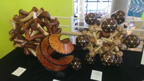
Day0054-11-02-15imag0538 — Sculpture at Bridges 2015 in Baltimore

Not just M. C. Escher, either (though many are interested in his work). Some Bridges attendees (shall we call them Bridgers?) are artists by profession, but others are mathematicians, computer scientists, physicists — you name it. All are artists by vocation.

Interests span not only art in a more usual sense — watercolor, acrylic, oil, pastel, drawing — but also digital art, sculpture in almost any medium you can think of, poetry, architecture, music, fiber arts, dance, digital animations and movies, fashion, origami, and likely there will be some new art form introduced this summer as well!

The art exhibition is amazing. You can see a few examples above. You see the wooden spiral? Each inlaid rectangle is a different piece of wood! The craftsmanship is really superb.

One neat aspect is that most of the artists also attend Bridges. That means if you see something you really like, you can just look for the right name tag and start up a conversation. As you would expect, all the artists are eager to discuss their work.

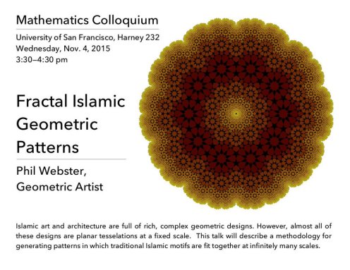
Be ready for some surprises, too. I met my friend Phil Webster at the conference – we starting talking because I was from San Francisco, and he also lives in the Bay area. So we’ve met up a few times since the conference to discuss mathematics, art, and programming. He even gave a talk in our Mathematics Colloquium at the University of San Francisco. Of course, his talk was great….

CS-rZ1zUkAQoQ_i.jpg_large

Even if you don’t go to the conference, you can still appreciate all the art. You can visit the Bridges 2015 online gallery and see all the art that was exhibited. Not only are there descriptions of all the works by the artists themselves, but there’s also contact information so you can get in touch if you’d like. Please do!

The Bridges 2016 gallery is not online yet, but I’ve got two pieces accepted for this year’s exhibition. This is my favorite.

Spiral

Then there are the talks. You learn so much just by going to them. The range of topics is incredibly diverse — look back at the list above! Last summer, I gave a talk about Random Walks on Vertices of Archimedean Tilings. My favorite work discussed in the paper is Bear. You can read the paper to learn how it was made, if you’re interested. The first print of Bear is hanging in my friend Cory’s house in Florida. Hi, Cory!

Bear4Web

As you’ll see if you click on the link to my paper, there is an archive of all papers — over 1000! — given at Bridges conferences since 1998. What’s nice is that you can actually search for specific topics, so it’s easy to use. No shortage of reading material on mathematics and art….

In addition to the exhibition and all the presentations, there are also dance performances, poetry readings, theatre performances, movie showings, a music night — any number of interesting activities relating mathematics and art. If you want to learn more, just go to the Bridges 2016 website. There’s complete information on the upcoming conference there.

This year, the conference is being held at the University of Jyväskylä in Jyväskylä, Finland. I’ve never been to Finland before, so I’m looking forward to an exciting trip! What’s also nice about the conference is that in the evenings, you can just take a stroll with other Bridgers, looking for some interesting place to have dinner. I always love exploring new countries, and especially like trying new cuisines!

But even though Bridges 2016 is in July, I actually starting preparing last November. Since there was a January deadline for submitting papers to the conference, and since I knew I’d be doing a lot of traveling over our Winter Break, I wanted to get an early start. The papers are all reviewed by three referees, so your mathematics should be sound. Usually they have comments to make, and so you often need to make some revisions a few months later before a final submission.

My paper is on fractals this year. A lot of what I wrote in that paper you’ve already seen on my blog — but I’ll be sure to give a link when I write a follow-up post on Bridges 2016 later on in the summer. Here’s one of my favorite images discussed in the paper.

koch090-150tweak

There are deadlines to submit artwork as well, so it’s important to be organized. For both papers and artwork, the online submission system is actually really easy to use. I just wanted to let you know something about the process so you can submit something to next year’s conference….

Last Fall, I received an email about a new addition to the Bridges menu — student scholarships. And in my calculus class, I had a student Nick who is a double major in mathematics and art.

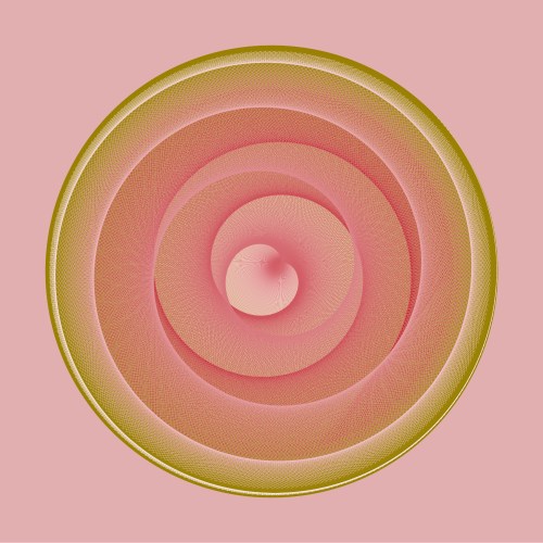
Turns out Nick was really interested in trying to submit to Bridges, so we worked out a one-credit directed study course just for that purpose. As of this moment, I’m happy to say that two of Nick’s artworks were accepted! And we just submitted the final revisions to his paper, and are waiting to hear back. We should know about the scholarship soon — I’ll update this post when I have more information. One of my favorite images from Nick’s paper is this one.

art4

You can read the paper to see how he creates it….link to follow.

So think about including Bridges in your future travel! Many artists bring their families and make a summer vacation out of the conference. It’s quite an experience.

And if you’re a student, consider submitting as well! Maybe you’ll earn a scholarship to attend: here’s more information on the Student Travel Scholarship. Preference is given to those student who submit papers, artwork, or movies.

You will need a letter from one of your teachers or professors — so ask someone to be your mentor. If you can’t find someone, well, just ask me. I’ll be glad to help out (as long as I don’t get too many requests!).

Later on in the summer, I’ll tell you all about the experience. Hope to see you at some Bridges conference soon!

P.S. (10 July 2106): Nick did receive the travel scholarship. Congratulations!