We had yet another amazing meeting of the Bay Area Mathematical Artists yesterday! Just two speakers — but even so, we went a half-hour over our usual 5:00 ending time.
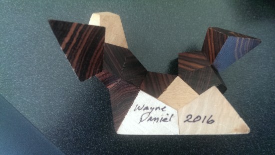
Our first presenter was Stan Isaacs. There was no real title to his presentation, but he brought another set of puzzles from his vast collection to share. He was highlighting puzzles created by Wayne Daniel.
Below you’ll see one of the puzzles disassembled. The craftsmanship is simply remarkable.

If you look carefully, you’ll see what’s going on. The outer pieces make an icosahedron, and when you take those off, a dodecahedron, then a cube…a wooden puzzle of nested Platonic solids! The pieces all fit together so perfectly. Stan is looking forward to an exhibition of Wayne’s work at the International Puzzle Party in San Diego later on this year. For more information, contact Stan at stan@isaacs.com.
Our second speaker was Scott Kim (www.scottkim.com), who’s presentation was entitled Motley Dissections. What is a motley dissection? The most famous example is the problem of the squared square — that is, dissecting a square with an integer side length into smaller squares with integer side lengths, but with all the squares different sizes.
One property of such a dissection is that no two edges of squares meet exactly corner to corner. In other words, edges always overlap in some way.
But there are of course many other motley dissections. For example, below you see a motley dissection of one rectangle into five, one pentagon into eleven, and finally, one hexagon into a triangle, square, pentagon and hexagon.
 Look carefully, and you’ll see that no single edge in any of these dissections exactly matches any other. For these decompositions, Scott has proved they are minimal — so, for example, there is no motley dissection of one pentagon to ten or fewer. The proofs are not exactly elegant, but they serve their purpose. He also mentioned that he credits Donald Knuth with the term motley dissection, who used the term in a phone conversation not all that long ago.
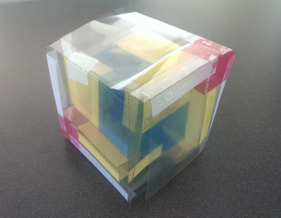
Can you cube the cube? That is, can you take a cube and subdivide it into cubes which are all different? Scott showed us a simple proof that you can’t. But, it turns out, you can box the box. In other words, if the length, width, and height of the larger box and all the smaller boxes may be different, then it is possible to box the box.
Next week, Scott is off to the Gathering 4 Gardner in Atlanta, and will be giving his talk on Motley Dissections there. He planned an activity where participants actually build a boxed box — and we were his test audience!
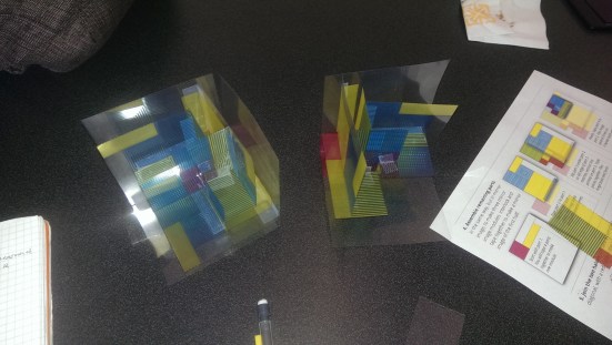
He created some very elaborate transparencies with detailed instructions for cutting out and assembling. There were a very few suggestions for improvement, and Scott was happy to know about them — after all, it is rare that something works out perfectly the first time. So now, his success at G4G in Atlanta is assured….
We were so into creating these boxed boxes, that we happily stayed until 5:30 until we had two boxes completed.
I should mention that Scott also discussed something he terms pseudo-duals in two, three, and even four dimensions! There isn’t room to go into those now, but you can contact him through his website for more information.
As usual, we went out to dinner afterwards — and we gravitated towards our favorite Thai place again. The dinner conversation was truly exceptional this evening, revolving around an animated conversation between Scott Kim and magician Mark Mitton (www.markmitton.com).
The conversation was concerned with the way we perceive mathematics here in the U.S., and how that influences the educational system. Simply put, there is a lot to be desired.
One example Scott and Mark mentioned was the National Mathematics Festival (http://www.nationalmathfestival.org). Tens of thousands of kids and parents have fun doing mathematics. Then the next week, they go back to their schools and keep learning math the same — usually, unfortunately, boring — way it’s always been learned.
So why does the National Mathematics Festival have to be a one-off event? It doesn’t! Scott is actively engaged in a program he’s created where he goes into an elementary school at lunchtime one day a week and let’s kids play with math games and puzzles.
Why this model? Teachers need no extra prep time, kids don’t need to stay after school, and so everyone can participate with very little needed as far as additional resources are concerned. He’s hoping to create a package that he can export to any school anywhere where with minimal effort, so that children can be exposed to the joy of mathematics on a regular basis.
Mark was interested in Scott’s model: consider your Needs (improving the perception of mathematics), be aware of the Forces at play (unenlightened administrators, for example, and many other subtle forces at work, as Mark explained), and then decide upon Actions to take to move the Work (applied, pure, and recreational mathematics) forward.
The bottom line: we all know about this problem of attitudes toward mathematics and mathematics education, but no one really knows what to do about it. For Scott, it’s just another puzzle to solve. There are solutions. And he is going to find one.
We talked for over two hours about these ideas, and everyone chimed in at one time or another. Yes, my summary is very brief, I know, but I hope you get the idea of the type of conversation we had.
Stay tuned, since we are planning an upcoming meeting where we focus on Scott’s model and work towards a solution. Another theme throughout the conversation was that mathematics is not an activity done in isolation — it is a communal activity. So the Needs will not be addressed by a single individual, rather a group, and likely involving many members of many diverse communities.
A solution is out there. It will take a lot of grit to find it. But mathematicians have got grit in spades.


 or
or  is involved;
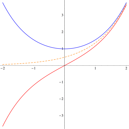
 is shown in blue, and the graph of
  is shown in red. The dashed orange graph is
  which is easily seen to be asymptotic to both graphs.
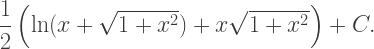
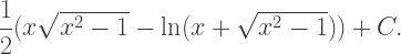
 is an even function, just like
 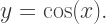 Similarly,

 lies on a unit hyperbola, much like
  lies on a unit circle.
 Recall that given any function
  we may define
 respectively.


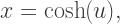
 to
to  to
to  sometimes changes of sign are necessary.

 and
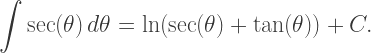
and  Gone are the days of remembering signs when differentiating and integrating trigonometric functions! This is one feature of hyperbolic trigonometric functions which students always appreciate….

 for
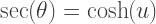
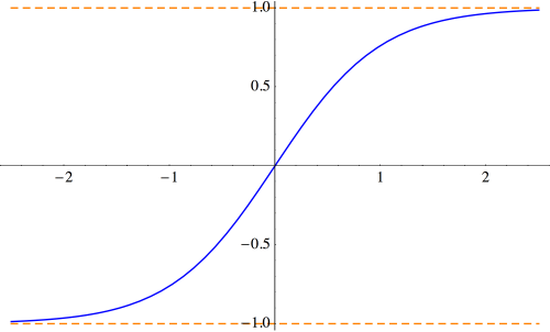
for  Begin with the definition:


 is always negative, so that we must choose the positive sign. Thus,
 or
or  These get students working with the definitions and thinking about asymptotic behavior.
 where it crosses the x-axis at
  we simply retain the
  term and substitute the root
  into the other terms, getting

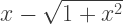
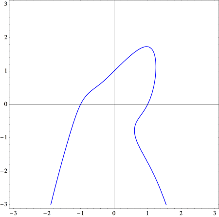
 (the U-shaped piece, since the sideways U-shaped piece involves writing
  as a function of
  ) is
) is  as shown below.
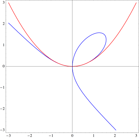

 and so rewrite the equation for the Folium of Descartes by using the substitution
  which results in
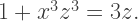
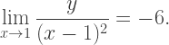
 we have
  giving us a good quadratic approximation at the origin.
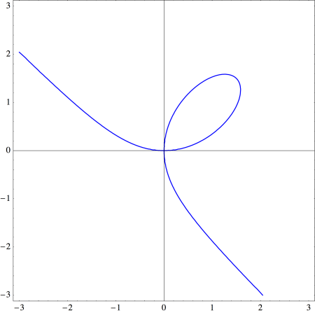
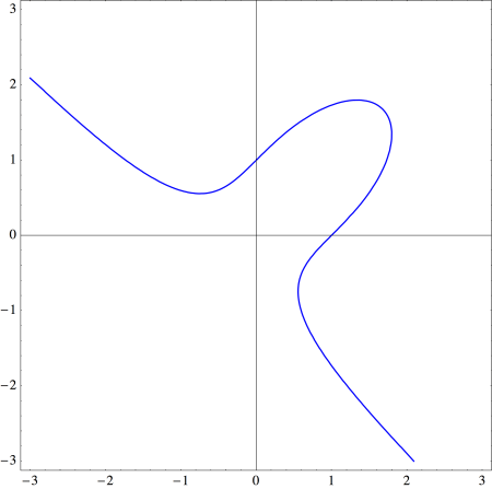
 looking at the curve

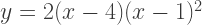
 with
with  yet to be determined. This results in
 we have
 Thus, in our case with
  we see that
  is a good approximation to the curve near the origin. The graph below shows just how good an approximation it is.
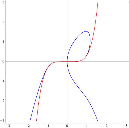

 which results in
 here. But if we move the
  to the other side and factor, we get
 to obtain
 And sure enough, the line
  does the trick:
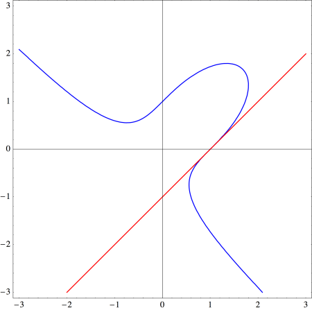


 This results in
 is even, since there is always a root at
  in this case. Here, we make the substitution
 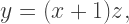 move the
  resulting in
 is a factor of
  so we have

 as well! This is a curious coincidence, for which I have no nice geometrical explanation. The case when
  is illustrated below.
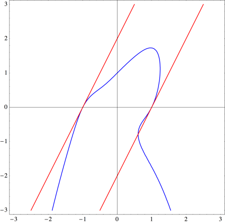

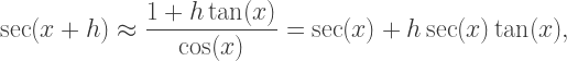
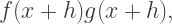
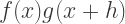
 Today, we’ll look at some more examples, and then derive the product, quotient and chain rules.

 as small as we like, and so approximate by considering
  as the sum of an infinite series:
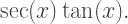
 We first factor the denominator:
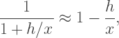


 so we replace each factor with its linear approximation:


 (or perhaps
 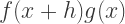 ). I have found that there is just no way to convincingly motivate this step. Yes, those of us who have seen it crop up in various forms know to try such tricks, but the typical first-time student of calculus is mystified by that mysterious step. Using linear approximations, there is absolutely no mystery at all.
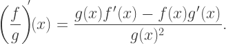
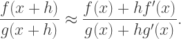


 and
and  but note that this involves using the chain rule to differentiate
  or (2) the mysterious “adding and subtracting the same expression” in the numerator. Using linear approximations avoids both.
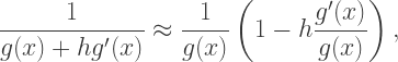
 is differentiable, it is also continuous, so this poses no real problem. Yes, perhaps there is a little hand-waving here, but in my opinion, no rigor is really lost.
 is differentiable, then
  exists, and so we can make
  as small as we like, so the “
 ” term acts like the “

