Last week, I ended with a sample exam I might give a calculus course which included both Skills problems and Conceptual problems. Before presenting the final installment of this series on assessment, I thought I’d take a few moments to discuss the genesis of this exam format.
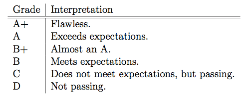
Again, the assumption here is that we are working in a more traditional system, where students must be assigned grades, and these grades must in large part be based on performance on exams.
Given IMSA’s statements about the advanced nature of their curriculum, I had concerns about the fairly traditional exams we gave in mathematics. In my mind, there was little to distinguish our exams from those given in any other rigorous calculus course.
The reason given to me by other mathematics faculty was that there just wasn’t time in a roughly hour-long exam to assess conceptual understanding. I wasn’t convinced, and I started thinking of an alternative. I did agree, however, that it wouldn’t work to have a conceptual question on an exam which might take half the exam period for a significant fraction of the students to complete.
What I finally settled upon was including a range of conceptual problems for which students only needed to provide a reasonable approach to solving. If you chose a conceptual problem which happened to be centered on a student’s weakness, you wouldn’t be able to assess a broader conceptual understanding. And if you insisted the problem be worked completely through, you encountered significant time constraints.
I’d like to share one last anecdote. I recall a parent visitation day one Saturday, which happened to be the day after I gave a calculus exam. Two of the parents approached me after the session and told me how much their son or daughter enjoyed my exam. This indicated to me that for the student who can perform the routine procedures easily, they want to be challenged to think outside the box, and indeed they thrive on such challenge. Shouldn’t we, as educators, find ways to stimulate all of our students, rather than be content with having students in the middle earn their B’s, making sure the struggling students earn their C’s, and relegating the very capable students to a sustained boredom?
And now for the last installment….
“Where does this bring us? Here are some key points as I see them.
- We should move away from assigning grades punitively.
- We should reconsider the “point'”system of evaluating student performance. Referring to the TIMSS (Third International Mathematics and Science Study): “In our study, teachers were asked what ‘main thing’ they wanted students to learn from the lesson. Sixty-one percent of U.S. teachers described skills they wanted their students to learn. They wanted students to be able to perform a procedure, solve a particular kind of problem, and so on….On the same questionnaire, 73 percent of Japanese teachers said that the main thing they wanted their students to learn from the lesson was to think about things in a new way, such as to see new relationships between mathematical ideas.” (Stigler and Hiebert, The Teaching Gap, ISBN 0-684-85274-8, pp. 89-90.) A point system reflects the assessment of procedural knowledge.
- “We can think of all assessment uses as falling into one of two general categories — assessments FOR learning and assessments OF learning.” (From an internal document distributed to mathematics teachers at IMSA.) But why? The distinction is artificial. There are many other ways to compartmentalize assessments, such as timed/untimed, individual/group, skill/conceptual, procedural/relational, short-term/long-term, etc. The main argument for focusing on the “for/or” distinction is its relationship to student motivation — but we are given no context for it. I suggest that our typical IMSA student is highly motivated — certainly in relation to the average student in a typical high school classroom.
- We should consider the assignment of letter grades in general. Right now, it would be impractical to suggest that we have formal written evaluations of each student in each class. But is it desirable? And if so, what resources are necessary to support such a system?
- We should discuss the assessment of problem-solving.
Will any of these suggestions help to illuminate the power of ideas? I’m not sure. With the current need to assign grades, and their current cultural meaning and importance — especially when it comes to applying to college — there will be the necessary compromises in the classroom. I realize that many suggestions are of the “move away” rather than the “move toward” type. But I suppose that if there is something I am moving toward, it’s giving students at all levels more of a BC Fast-Track experience regardless of the depth of content.
This means actively moving toward a classroom environment where earning good grades is subordinate to learning complex concepts. Of course the two are not mutually exclusive — but I’d rather have students earn good grades because they learned, rather than learn in order to get good grades.
Of course many issues brought up in these remarks have been left hanging or only tentatively developed. These brief comments are meant to suggest questions for discussion, not definitive answers.
I can’t resist ending with the following challenge from Maslow: “In order to be able to choose in accord with his own nature and develop it, the child must be permitted to retain the subjective experiences of delight and boredom, as the criteria of the correct choice for him. The alternative criterion is making the choice in terms of the wish of another person. The Self is lost when this happens. (Maslow, source cited earlier, p. 58.) Is it possible to create a mathematics curriculum which can survive this test of course selection?”
Thanks for staying with this series! No, there is no simple resolution to any of the issues described in this essay. But that doesn’t mean we shouldn’t be involved in a conversation about them….

 find
find 


 at
at 
 and
and  are differentiable functions. Find


 is tangent to both
  and
and  Find
Find  and
and 


 by the cubic polynomial
 the natural logarithm? There are a few different ways this is usually shown, but here’s one I haven’t seen before: consider the limit


 I’m so conditioned to thinking of
  as a constant that I never thought of turning it into the variable. It’s a nice proof.
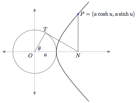
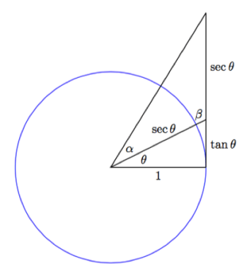
 The goal of this exercise is to find a geometrical interpretation of the relationship
 and consider the point
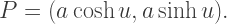
 on the x-axis to the point
  Next, draw a tangent from
  to the auxiliary circle, meeting it at
  Finally, join
  to the origin.
 is tangent to the circle, we know that
  is a right triangle. Therefore
  But by construction,
  and so


 amounts to multiplying the function by
  and increasing the angle in the sine function by
  Therefore
![[a,b],](https://s0.wp.com/latex.php?latex=%5Ba%2Cb%5D%2C&bg=ffffff&fg=333333&s=2&c=20201002) divide the interval into six equal subintervals with points
divide the interval into six equal subintervals with points  and corresponding function values
  Then
Then

![[a,x].](https://s0.wp.com/latex.php?latex=%5Ba%2Cx%5D.&bg=ffffff&fg=333333&s=2&c=20201002) In other words, we want to find weights
In other words, we want to find weights 
 and
and  such that
 and
and  about the point
  The first is easy using the Fundamental Theorem of Calculus, assuming sufficient differentiability:
 we need to evaluate several derivatives at
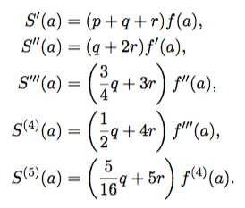
 as possible. This will make the derivatives of
  and
and  match, and the Taylor polynomials will be equal up to some order.
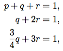

 and
and  Note that these values also imply that


 to create an approximation

 and solve the first six equations in terms of
  This gives us

 which is in the interval just described. This gives the sequence of weights to be
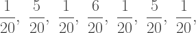
 and you notice that all divisions are by 10. Can you see the advantage? If you have a table of values for your functions, you just need to multiply function values by a single-digit number, and then move the decimal place over one. An approximators dream!
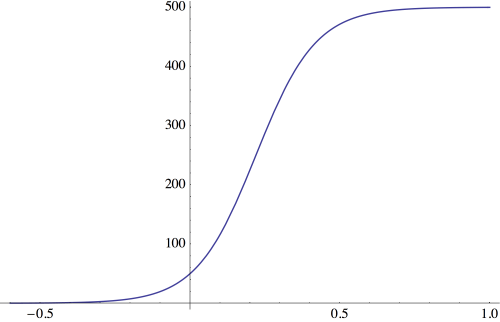
 is a constant which influences how fast the population grows, and
  is called the carrying capacity of the environment.
 and so the population growth is almost exponential. But when
  gets very close to
  then
then  and so population growth slows down. And of course when
  growth stops — hence calling
 and
and 


 and
and  to write
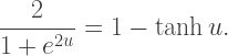
 and
and  we need to scale by a factor of
  so that the asymptotes of the logistic curve are
 and
and 
 We can accomplish this be replacing
  with
with 


 is an odd function, becomes
 might be suggested, but how would we relate this to the exponential function?
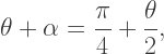
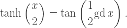
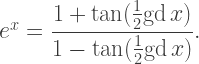
 using the hyperbolic trigonometric substitution
  Today, we’ll look at this substitution in more depth.
 and
and  is described by the gudermannian function, defined by
 so that this relationship is in fact invertible.
 to obtain the quadratic

 then
then  must be an increasing function of
  It is not difficult to see that we must choose “plus,” so that
  and consequently
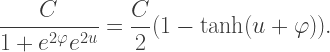
 by
by  in order to form an isosceles triangle. Thus,
 observe that
  is supplementary to both
  and
and  so that


 giving
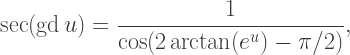


 giving
 Again using the usual circular trigonometric identities, we can show that
 and
and 
 is the inverse of the gudermannian function, then
