Day146 – Creativity in Mathematics

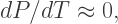
Of course, there is always more to say about hyperbolic trigonometry…. Next, we’ll look at what is usually called the logistic curve, which is the solution to the differential equation

$\dfrac{dP}{dt}=kP(C-P),\quad P(0)\ \text{given}.$

The logistic curve comes up in the usual chapter on differential equations, and is an example of population growth. Without going into too many details (since the emphasis is on hyperbolic trigonometry), $k$ is a constant which influences how fast the population grows, and $C$ is called the carrying capacity of the environment.

Note that when $P$ is very small, $C-P\approx C,$ and so the population growth is almost exponential. But when $P(t)$ gets very close to $C,$ then $dP/dT\approx0,$ and so population growth slows down. And of course when $P(t)=C,$ growth stops — hence calling $C$ the carrying capacity of the environment. It represents the largest population the environment can sustain.

Here is an example of such a curve where $C=500,$ $k=0.02,$ and $P(0)=50.$

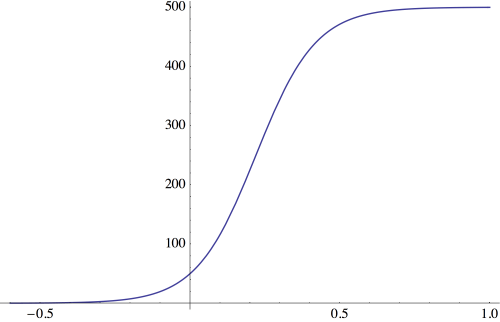
Notice the S shape, obtained from a curve rapidly growing when the population is small. It happens that the population grows fastest at half the carrying capacity, and then growth slows to zero as the carrying capacity is reached.

Skipping the details (simple separation of variables), the solution to this differential equation is given by

$P(t)=\dfrac{C}{1+Ae^{-kCt}},\qquad A=\dfrac{C-P(0)}{P(0)}.$

I will digress for a moment, however, to mention partial fractions (as I step on my calculus soapbox). I have mentioned elsewhere that incomprehensible chapter in calculus textbooks: Techniques of Integration. Pedagogically a disaster for so many reasons.

The first time I address partial fractions is when summing telescoping series, such as

$\displaystyle\sum_{n=1}^\infty\dfrac1{n(n+1)}.$

It really is necessary. But I only go so far as to be able to sum such series. (Note: I do series as the middle third of Calculus II, rather than the end. A colleague suggested that students are more tired near the end of the course, which is better for a more technique-oriented discussion of the solution to differential equations, which typically comes before series.)

You also need partial fractions to solve the differential equation for the logistic curve, which is when I revisit the topic. After finding the logistic curve, we talk about partial fractions in more detail. The point is that students see some motivation for the method of partial fractions — which they decidedly don’t in a chapter on techniques of integration.

OK, time to step off the soapbox and talk about hyperbolic trigonometry…. The punch line is that the logistic curve is actually a scaled and shifted hyperbolic tangent curve! Of course it looks like a hyperbolic tangent, but let’s take a moment to see why.

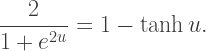
We first use the definitions of $\sinh u$ and $\cosh u$ to write

$\tanh u=\dfrac{\sinh h}{\cosh u}=1-\dfrac2{1+e^{2u}}.$

This results in

$\dfrac2{1+e^{2u}}=1-\tanh u.$

You can see the form of the equation of the logistic curve starting to take shape. Since the hyperbolic tangent has horizontal tangents at $y=-1$ and $y=1,$ we need to scale by a factor of $C/2$ so that the asymptotes of the logistic curve are $C$ units apart:

$\dfrac C{1+e^{2u}}=\dfrac{C}2\left(1-\tanh u\right).$

Note that this puts the horizontal asymptotes of the function at $y=0$ and $y=C.$

To take into account the initial population, we need a horizontal shift, since otherwise the initial population would be $C/2.$ We can accomplish this be replacing $\tanh u$ with $\tanh(u+\varphi):$

$\dfrac C{1+e^{2\varphi} e^{2u}}=\dfrac C2(1-\tanh(u+\varphi)).$

We’re almost done at this point: we simply need

$e^{2\varphi}=A,\qquad 2u=-kCt.$

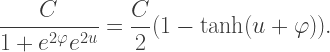
Solving and substituting back results in

$P(t)=\dfrac C2\left(1-\tanh\left(\dfrac{-kCt+\ln A}2\right)\right),$

which, since $\tanh$ is an odd function, becomes

$P(t)=\dfrac C2\left(1+\tanh\left(\dfrac{kCt-\ln A}2\right)\right).$

And there it is! The logistic curve as a scaled, shifted hyperbolic tangent.

Now what does showing this accomplish? I can’t give you a definite answer from the point of view of the students. But for me, it is a way to tie two seemingly unrelated concepts — hyperbolic trigonometry and solution of differential equations by separation of variables — together in a way that is not entirely contrived (as so many calculus textbook problems are).

I would love to perform the following experiment: work out the solution to the differential equation together as a guided discussion, and then prompt students to suggest functions this curve “looks like.” Of course the $\arctan$ might be suggested, but how would we relate this to the exponential function?

Eventually we’d tease out the hyperbolic tangent, since this function actually does involve the exponential function. Then I’d move into an inquiry-based lesson: give the students the equation of a logistic curve, and have them work out the conversion to the hyperbolic tangent.

And as is typical in such an approach, I would put students into groups, and go around the classroom and nudge them along. See what happens.

I say that yes, calculus students should be able to do this. I recently sent an email about pedagogy in calculus which, among other things, addressed the question: What do calculus students really need to know?

There is no room to adequately address that important question here, but in today’s context, I would say this: I think it is more important for a student to be able to rewrite $P(t)$ as a hyperbolic tangent than it is for them to know how to sketch the graph of $P(t).$

Why? Because it is trivial to graph functions, now. Type the formula into Desmos. But how to interpret the graph? Rewrite it? Analyze it? Draw conclusions from it? We need to focus on what is no longer necessary, and what is now indispensable. To my knowledge, no one has successfully done this.

I think it is about time for that to change….

Tag: Day146

Calculus: Hyperbolic Trigonometry, IV