March 2018 – Creativity in Mathematics

Calculus: Linear Approximations, I

Last week’s post on the Geometry of Polynomials generated a lot of interest from folks who are interested in or teach calculus. So I thought I’d start a thread about other ideas related to teaching calculus.

This idea is certainly not new. But I think it is sorely underexploited in the calculus classroom. I like it because it reinforces the idea of derivative as linear approximation.

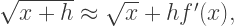
The main idea is to rewrite

$\displaystyle\lim_{h\to 0}\dfrac{f(x+h)-f(x)}h=f'(x)$

$f(x+h)\approx f(x)+hf'(x),$

with the note that this approximation is valid when $h\approx0.$ Writing the limit in this way, we see that $f(x+h),$ as a function of $h,$ is linear in $h$ in the sense of the limit in the definition actually existing — meaning there is a good linear approximation to $f$ at $x.$

Moreover, in this sense, if

$f(x+h)\approx f(x)+hg(x),$

then it must be the case that $f'(x)=g(x).$ This is not difficult to prove.

Let’s look at a simple example, like finding the derivative of $f(x)=x^2.$ It’s easy to see that

$f(x+h)=(x+h)^2=x^2+h(2x)+h^2.$

So it’s easy to read off the derivative: ignore higher-order terms in $h,$ and then look at the coefficient of $h$ as a function of $x.$

Note that this is perfectly rigorous. It should be clear that ignoring higher-order terms in $h$ is fine since when taking the limit as in the definition, only one $h$ divides out, meaning those terms contribute $0$ to the limit. So the coefficient of $h$ will be the only term to survive the limit process.

Also note that this is nothing more than a rearrangement of the algebra necessary to compute the derivative using the usual definition. I just find it is more intuitive, and less cumbersome notationally. But every step taken can be justified rigorously.

Moreover, this method is the one commonly used in more advanced mathematics, where functions take vectors as input. So if

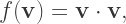
$f({\bf v})={\bf v}\cdot{\bf v},$

we compute

$f({\bf u}+h{\bf v})={\bf u}\cdot{\bf u}+2h{\bf u}\cdot{\bf v}+h^2{\bf v}\cdot{\bf v},$

and read off

$\nabla_{\bf v}f({\bf u})=2{\bf u}\cdot{\bf v}.$

I don’t want to go into more details here, since such calculations don’t occur in beginning calculus courses. I just want to point out that this way of computing derivatives is in fact a natural one, but one which you don’t usually encounter until graduate-level courses.

Let’s take a look at another example: the derivative of $f(x)=\sin(x),$ and see how it looks using this rewrite. We first write

$\sin(x+h)=\sin(x)\cos(h)+\cos(x)\sin(h).$

Now replace all functions of $h$ with their linear approximations. Since $\cos(h)\approx1$ and $\sin(h)\approx h$ near $h=0,$ we have

$\sin(x+h)\approx\sin(x)+h\cos(x).$

This immediately gives that $\cos(x)$ is the derivative of $\sin(x).$

Now the approximation $\cos(h)\approx1$ is easy to justify geometrically by looking at the graph of $\cos(x).$ But how do we justify the approximation $\sin(h)\approx h$ ?

Of course there is no getting around this. The limit

$\displaystyle\lim_{h\to0}\dfrac{\sin(h)}h$

is the one difficult calculation in computing the derivative of $\sin(x).$ So then you’ve got to provide your favorite proof of this limit, and then move on. But this approximation helps to illustrate the essential point: the differentiability of $\sin(x)$ at $x=0$ does, in a real sense, imply the differentiability of $\sin(x)$ everywhere else.

So computing derivatives in this way doesn’t save any of the hard work, but I think it makes the work a bit more transparent. And as we continually replace functions of $h$ with their linear approximations, this aspect of the derivative is regularly being emphasized.

How would we use this technique to differentiate $f(x)=\sqrt x$ ? We need

$\sqrt{x+h}\approx\sqrt x+hf'(x),$

and so

$x+h\approx \left(\sqrt x+hf'(x)\right)^2\approx x+2h\sqrt xf'(x).$

Since the coefficient of $h$ on the left is $1,$ so must be the coefficient on the right, so that

$2\sqrt xf'(x)=1.$

As a last example for this week, consider taking the derivative of $f(x)=\tan(x).$ Then we have

$\tan(x+h)=\dfrac{\tan(x)+\tan(h)}{1-\tan(x)\tan(h)}.$

Now since $\sin(h)\approx h$ and $\cos(h)\approx 1,$ we have $\tan(h)\approx h,$ and so we can replace to get

$\tan(x+h)\approx\dfrac{\tan(x)+h}{1-h\tan(x)}.$

Now what do we do? Since we’re considering $h$ near $0,$ then $h\tan(x)$ is small (as small as we like), and so we can consider

$\dfrac1{1-h\tan(x)}$

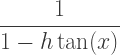
as the sum of the infinite geometric series

$\dfrac1{1-h\tan(x)}=1+h\tan(x)+h^2\tan^2(x)+\cdots$

Replacing, with the linear approximation to this sum, we get

$\tan(x+h)\approx(\tan(x)+h)(1+h\tan(x)),$

and so

$\tan(x+h)\approx\tan(x)+h(1+\tan^2(x)).$

This give the derivative of $\tan(x)$ to be

$1+\tan^2(x)=\sec^2(x).$

Neat!

Now this method takes a bit more work than just using the quotient rule (as usually done). But using the quotient rule is a purely mechanical process; this way, we are constantly thinking, “How do I replace this expression with a good linear approximation?” Perhaps more is learned this way?

There are more interesting examples using this geometric series idea. We’ll look at a few more next time, and then use this idea to prove the product, quotient, and chain rules. Until then!

The Geometry of Polynomials

I recently needed to make a short demo lecture, and I thought I’d share it with you. I’m sure I’m not the first one to notice this, but I hadn’t seen it before and I thought it was an interesting way to look at the behavior of polynomials where they cross the x-axis.

The idea is to give a geometrical meaning to an algebraic procedure: factoring polynomials. What is the geometry of the different factors of a polynomial?

Let’s look at an example in some detail: $f(x)=2(x-4)(x-1)^2.$ poly0b

Now let’s start looking at the behavior near the roots of this polynomial.

poly0c

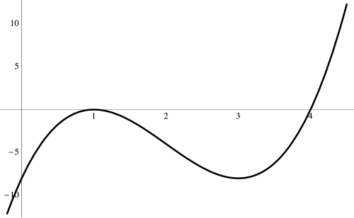
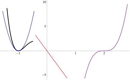
Near $x=1,$ the graph of the cubic looks like a parabola — and that may not be so surprising given that the factor $(x-1)$ occurs quadratically.

poly0d

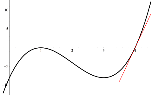
And near $x=4,$ the graph passes through the x-axis like a line — and we see a linear factor of $(x-4)$ in our polynomial.

But which parabola, and which line? It’s actually pretty easy to figure out. Here is an annotated slide which illustrates the idea.

Day137poly1

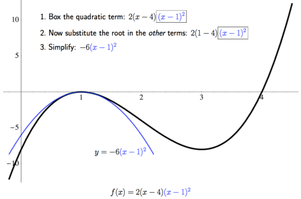
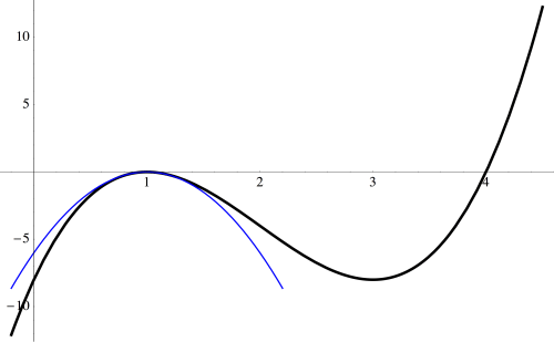
All you need to do is set aside the quadratic factor of $(x-1)^2,$ and substitute the root, $x=1,$ in the remaining terms of the polynomial, then simplify. In this example, we see that the cubic behaves like the parabola $y=-6(x-1)^2$ near the root $x=1.$ Note the scales on the axes; if they were the same, the parabola would have appeared much narrower.

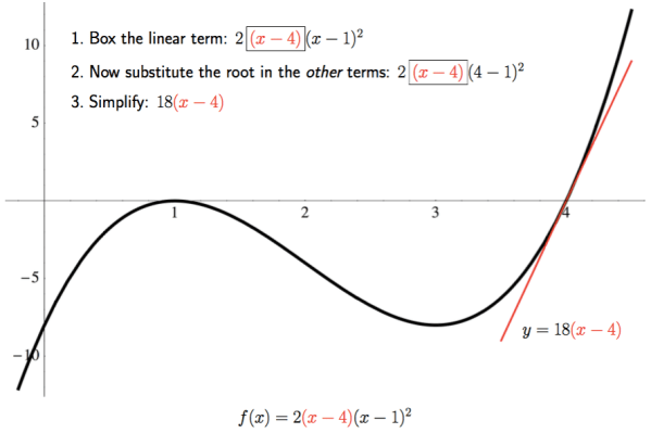
We perform a similar calculation at the root $x=4.$

Day137poly2

Just isolate the linear factor $(x-4),$ substitute $x=4$ in the remaining terms of the polynomial, and then simplify. Thus, the line $y=18(x-4)$ best describes the behavior of the graph of the polynomial as it passes through the x-axis. Again, note the scale on the axes.

We can actually use this idea to help us sketch graphs of polynomials when they’re in factored form. Consider the polynomial $f(x)=x(x+1)^2(x-2)^3.$ Begin by sketching the three approximations near the roots of the polynomial. This slide also shows the calculation for the cubic approximation.

Now you can begin sketching the graph, starting from the left, being careful to closely follow the parabola as you bounce off the x-axis at $x=-1.$

poly1d

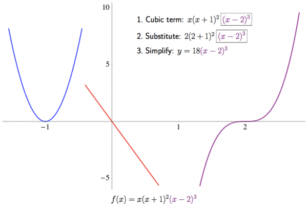
Continue, following the red line as you pass through the origin, and then the cubic as you pass through $x=2.$ Of course you’d need to plot a few points to know just where to start and end; this just shows how you would use the approximations near the roots to help you sketch a graph of a polynomial.

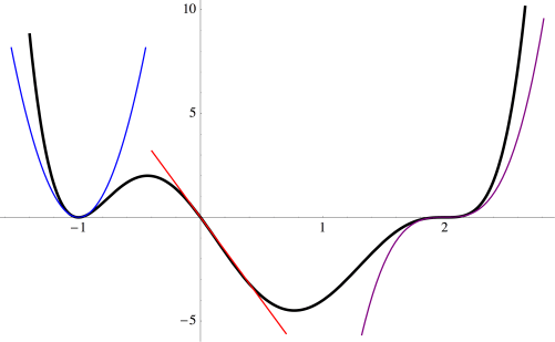
poly1f

Why does this work? It is not difficult to see, but here we need a little calculus. Let’s look, in general, at the behavior of $f(x)=p(x)(x-a)^n$ near the root $x=a.$ Given what we’ve just been observing, we’d guess that the best approximation near $x=a$ would just be $y=p(a)(x-a)^n.$

Just what does “best approximation” mean? One way to think about approximating, calculuswise, is matching derivatives — just think of Maclaurin or Taylor series. My claim is that the first $n$ derivatives of $f(x)=p(x)(x-a)^n$ and $y=p(a)(x-a)^n$ match at $x=a.$

First, observe that the first $n-1$ derivatives of both of these functions at $x=a$ must be 0. This is because $(x-a)$ will always be a factor — since at most $n-1$ derivatives are taken, there is no way for the $(x-a)^n$ term to completely “disappear.”

But what happens when the $n$ th derivative is taken? Clearly, the $n$ th derivative of $p(a)(x-a)^n$ at $x=a$ is just $n!p(a).$ What about the $n$ th derivative of $f(x)=p(x)(x-a)^n$ ?

Thinking about the product rule in general, we see that the form of the $n$ th derivative must be $f^{(n)}(x)=n!p(x)+ (x-a)(\text{terms involving derivatives of } p(x)).$ When a derivative of $p(x)$ is taken, that means one factor of $(x-a)$ survives.

So when we take $f^{(n)}(a),$ we also get $n!p(a).$ This makes the $n$ th derivatives match as well. And since the first $n$ derivatives of $p(x)(x-a)^n$ and $p(a)(x-a)^n$ match, we see that $p(a)(x-a)^n$ is the best $n$ th degree approximation near the root $x=a.$

I might call this observation the geometry of polynomials. Well, perhaps not the entire geometry of polynomials…. But I find that any time algebra can be illustrated graphically, students’ understanding gets just a little deeper.

Those who have been reading my blog for a while will be unsurprised at my geometrical approach to algebra (or my geometrical approach to anything, for that matter). Of course a lot of algebra was invented just to describe geometry — take the Cartesian coordinate plane, for instance. So it’s time for algebra to reclaim its geometrical heritage. I shall continue to be part of this important endeavor, for however long it takes….

The Puzzle Archives, II

This week, I’ll continue with some more problems from the contests for the 2014 conference of the International Group for Mathematical Creativity and Giftedness. We’ll look at problems from the Intermediate Contest today. Recall that the first three problems on all contests were the same; you can find them here.

The first problem I’ll share is a “ball and urn” problem. These are a staple of mathematical contests everywhere.

You have 20 identical red balls and 14 identical green balls. You wish to put them into two baskets — one brown basket, and one yellow basket. In how many different ways can you do this if the number of green balls in either basket is less than the number of red balls?

Another popular puzzle idea is to write a problem or two which involve the year of the contest — in this case, 2014.

A positive integer is said to be fortunate if it is either divisible by 14, or contains the two adjacent digits “14” (in that order). How many fortunate integers n are there between 1 and 2014, inclusive?

The other two problems from the contest I’ll share with you today are from other contests shared with me by my colleagues.

In the figure below, the perimeters of three rectangles are given. You also know that the shaded rectangle is in fact a square. What is the perimeter of the rectangle in the lower left-hand corner?

Day136problem

I very much like this last problem. It’s one of those problems that when you first look at it, it seems totally impossible — how could you consider all multiples of 23? Nonetheless, there is a way to look at it and find the correct solution. Can you find it?

Multiples of 23 have various digit sums. For example, 46 has digit sum 10, while 8 x 23 = 184 has digit sum 13. What is the smallest possible digit sum among all multiples of 23?

You can read more to see the solutions to these puzzles. Enjoy!

Continue reading The Puzzle Archives, II

Bay Area Mathematical Artists, VI

As I mentioned last time, this meeting took place at Santa Clara University. As we have several participants in the South Bay area, many appreciated the shorter drive…it turns out this was the most well-attended event to date. Even better, thanks to Frank, the Mathematics and Computer Science Department at Santa Clara University provided wonderful pastries, coffee, and juice for all!

Our first speaker was Frank A. Farris, our host at Santa Clara University. (Recall that last month, he presented a brief preview of his talk.) His talk was about introducing a sound element into his wallpaper patterns.

In order to do this, he used frequencies based on the spectrum of hexagonal and square grids. It’s not important to know what this means — the main idea is that you get frequencies that are not found in western music.

Frank’s idea was to take his wallpaper patterns, and add music to them using these non-traditional frequencies. Here is a screenshot from one of his musical movies:

Day135AmaryllisPMG

Frank was really excited to let us know that the San Jose Chamber Orchestra commissioned work by composer William Susman to accompany his moving wallpaper patterns. The concert will take place in a few weeks; here is the announcement, so you are welcome to go listen for yourself!

Day135susman_farris invite_18

Frank has extensive information about his work on his website http://math.scu.edu/~ffarris/, and even software you can download to make your very own wallpaper patterns. Feel free to email him with any questions you might have at ffarris@scu.edu.

The second talk, Salvador Dali — Old and New, was given by Tom Banchoff, retired from Brown University. He fascinated us with the story of his long acquaintance with Salvador Dali. It all began with an interview in 1975 with the Washington Post about Tom’s work in visualizing the fourth dimension.

He was surprised to see that the day after the interview, the article Visual Images And Shadows From The Fourth Dimension in the next day’s Post, as well as a picture of Dali’s Corpus Hypercubus (1954).

Dali_Crucifixion_hypercube — Salvador Dali’s *Crucifixion (Corpus* *Hypercubus)*

But Tom was aware that Dali was very particular about giving permission to use his work in print, and knew that the Post didn’t have time to get this permission in such a short time frame.

The inevitable call came from New York — Dali wanted to meet Tom. He wondered whether Dali was simply perturbed that a photo of his work was used without permission — but luckily, that was not the reason for setting up the meeting at all. Dali was interested in creating stereoscopic oil paintings, and stereoscopic images were mentioned in the Post article.

Thus began Tom’s long affiliation with Dali. He mentioned meeting Dali eight or nine times in New York (Dali came to New York every Spring to work), three times in Spain, and once in France. Tom remarked that Dali was the most fascinating person he’d ever met — and that includes mathematicians!

Then Tom proceeded to discuss the genesis of Corpus Hypercubus. His own work included collaboration with Charles Strauss at Brown University, which included rendering graphics to help visualize the fourth dimension — but this was back in the 1960’s, when computer technology was at its infancy. It was a lot more challenging then than it would be today to create the same videos.

Day135net — Tom’s rendition of a hypercube net.

He also spent some time discussing a net for the hypercube, since a hypercube net is the geometrical basis for Dali’s Corpus Hypercubus. What makes understanding the fourth dimension difficult is imagining how this net goes together.

It is not hard to imagine folding a flat net of six squares to make a cube — but in order to do that, we need to fold some of the squares up through the third dimension. But to fold the hypercube net to make a hypercube without distorting the cubes requires folding the cubes up into a fourth spatial dimension.

This is difficult to imagine! Needless to say, this was a very interesting discussion, and challenged participants to definitely think outside the box.

Tom remarked that Dali’s interest in the hypercube was inspired by the work of Juan de Herrera (1530-1597), who was in turn inspired by Ramon Lull (1236-1315).

Tom also mentioned an unusual project Dali was interested in near the end of his career. He wanted to design a horse that when looked at straight on, looks like a front view of a horse. But when looked from the side, it’s 300 meters long! For more information, feel free to email Tom at banchoff@math.brown.edu.

Day135horse — Dali’s sketch of the horse.

Suffice it to say that we all enjoyed Frank’s and Tom’s presentations. The change of venue was welcome, and we hope to be at Santa Clara again in the future.

Following the talks, Frank generously invited us to his home for a potluck dinner! He provided lasagna and eggplant parmigiana, while the rest of us provided appetizers, salads, side dishes, and desserts.

As usual, the conversation was quite lively! We talked for well over two hours, but many of us had a bit of a drive, so we eventually needed to make our collective ways home.

Next time, on April 7, we’ll be back at the University of San Francisco. At this meeting, we’ll go back to shorter talks in order to give several participants a chance to participate. Stay tuned for a summary of next month’s talks!