April 2017 – Creativity in Mathematics

What is…Inversive Geometry?

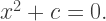
It’s been a while since we’ve looked at a new type of geometry, so today I’d like to introduce inversive geometry. Let’s look at a few pictures first for some motivation.

Day091a

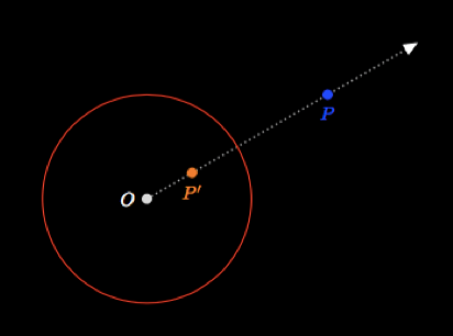
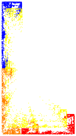
We would like to consider the operation of inverting points, as illustrated above. Suppose the red circle is a unit circle, the white dot is the origin, and consider the blue point P. Now define P′ (the orange dot) to be the inverse point of P as follows: draw a ray from the origin through P, and let P′ be that point on the ray such that

$[OP]\cdot[OP']=1,$

where $[AB]$ denotes the distance from A to B. That is, when you multiply the distances from the origin of a point and its inverse point, you get 1.

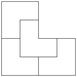
Now why would you want to do this? It turns out this operation is actually very interesting, and has many unexpected consequences. Consider the circles in the figure below.

Day091b

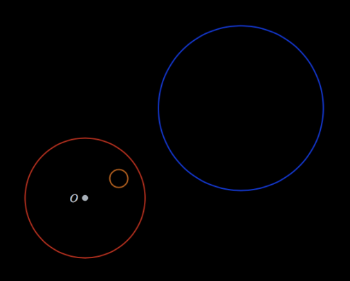
Start with the blue circle. Now for every point P on the blue circle, find its inverse point P′, and plot it in orange. The result is actually another circle! Yes, it works out exactly, although we won’t prove that here. Note that since every point on the blue circle is outside the unit circle (that is, greater than a distance of 1 from the origin), every inverse point on the orange circle must be inside the unit circle (that is, less than a distance of 1 from the origin).

This is just one geometrical property of inversion, and there are many others. I just want to suggest that the operation of inversion has many interesting properties.

If you pause a moment to think about this operation, you’ll notice there’s a little snag. Not every point has an inverse point. There’s just one point which is problematic here: the origin. According to the definition,

$[OO]\cdot[OO']=1.$

But the distance from the origin to itself is just 0, and it is not possible to multiply 0 by another number and get 1, since 0 times any real number is still 0.

Unless…could we somehow make the distance from O to O′ infinite? It should be clear that O′ cannot be a point in the plane different from the origin, since any point in the plane has a finite distance to the origin (just use the Pythagorean theorem).

So how do we solve this problem? We add another point to the usual Euclidean plane, called the point at infinity, which is usually denoted by the Greek letter ω.

You might be thinking, “Hey, wait a minute! You can’t just add a point because you need one. Where would you put it? The plane already extends out to infinity as it is!”

In a sense, that’s correct. But remember the idea of this thread — we’re exploring what geometry is. When we looked at taxicab geometry, we just changed the distance, not the points. And with spherical geometry, we looked at a very familiar geometrical object: the surface of a sphere. We can also change the points in our geometrical space.

How can we do this? Though perhaps a simplification, we must do this consistently as long as it is interesting.

What does this mean? In some sense, I can mathematically define lots of things. Let’s suppose I want to define a new operation on numbers, like this:

$a\otimes b=a^2+37b.$

Wow, we’ve just created something likely no one has thought of before! And yes, we probably have — and for good reason. This operation is not very interesting at all — no nice properties like commutativity or associativity, no applications that I can think of (what are you going to do with the 37?). But it is a perfectly legitimate arithmetical operation, defined for all real numbers a and b.

As I tried to suggest earlier, the operation of inversion is actually quite interesting. So it would be very nice to have a definition which allowed every point to have an inverse point.

But if we want to add ω, we must do so consistently. That is, the properties of ω cannot result in any contradictory statements or results.

It turns out that this is in fact possible — thought we do have to be careful. Although we can’t go into all the details of adding the point at infinity to the plane, here are some important properties that ω has:

The distance from ω to any other point in the plane is infinite;
ω lies on any unbounded curve (like a line or a parabola, but not a circle, for example);
The inverse point of ω is the origin; that is, O′ = ω and ω′ = O.

So we can create an entirely consistent system of geometry which contains all the points in the Euclidean plane plus a point at infinity which is infinitely far away from every other point. We usually call the Euclidean plane with ω added the extended plane.

With the new point, we can now say that every point in the extended plane has a unique inverse point.

This idea of adding a point at infinity is also important is other areas of mathematics. In considering the complex plane — that is, the set of points of the form a + bi, where i is a solution of the equation $x^2+1=0$ — it is often useful to add the number ∞, so that division by 0 is now possible. This results in the extended complex plane, and is very important in the study of complex analysis.

The point at infinity is also important in defining stereographic projection. Here, a sphere is placed on the plane, so that the South pole is the origin of the plane. The sphere is then projected onto the plane as follows: for any point on the sphere, draw a ray from the North pole through that point, and see where it intersects the plane.

Stereographic_projection_in_3D — Courtesy the *Wikipedia Commons.*

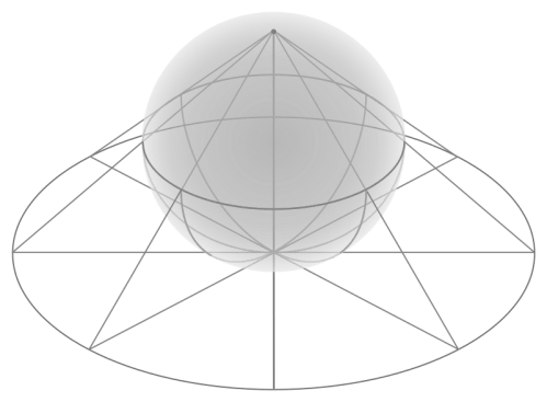
Where does the North pole get mapped to under this projection? Take one guess: the point at infinity!

So here is another new geometry! As we get introduced to more and more various geometrical systems, I hope you will continue to deepen your intuition about the question, What is a geometry?

Mathematics and Digital Art: Update 3

It’s hard to believe it’s been a month since my last update! This semester has been unusually busy.

At the end of my last update, I said I’d talk more about using L-systems in class. I decided to focus on the symmetrical Koch-like images I had been working on for the past few years. There are two reasons for this. First, it’s fresh — and demonstrates that creating new fractal images is an active research topic; not everything is known. Second, you need to know some elementary number theory in order to create symmetrical images. Since none of the mathematics we studied so far was closely related to number theory, this was a great opportunity to see yet another application of a different branch of mathematics.

Day007koch-45-175

I started with introducing the basics of modular arithmetic. This was new to most students, but the motivation was easy: the direction you’re pointing after any given move is relevant to deciding if your sequence of segments closes up. And any time you turn counterclockwise, you increment the direction by the angle you turn, but subtract 360° when you go over 360° since a turn of 360° doesn’t alter your direction. This is just using a modulus of 360 for the direction you’re pointing.

Then, I reminded them how to find the prime factorization of numbers in order to create a 2-adic valuation. Recall that the 2-adic valuation of a number is the exponent of the highest power of 2 which divides that number. This is significant since the 2-adic valuation (mod 2) indicates how to turn when drawing a Koch-like curve: a 0 represents one angle (60° for the Koch curve), and a 1 represents the other (240° for the Koch curve). So we created charts like this:

Day0902adic

Then finally, I showed students how to find angle pairs which created symmetrical images using a theorem in a paper I’m working on for the College Mathematics Journal. As the proof involves significantly more mathematics at a level beyond what we could reasonably discuss in the course, I just showed them the result. I won’t go into details here, but I’d be glad to share a draft of the paper if you’re interested and adventurous….

For their project work, they had to create images using the results of the theorem in Processing. Karla created this image, which I find interesting since it exhibits six-fold symmetry, but the exterior elements have seven points on them. So rarely do you encounter 6 and 7 together in geometry.

Day090karla

Peyton created this image, which is suggestive of a complete image, but which doesn’t include all the line segments. But the overall symmetry of the image is clear; you can complete it in your mind’s eye.

Day090Peyton

I also asked students to create an image which did not close up, to experiment with parameters which generated a more chaotic image. Colette created this image, which reminded her of the top of a pine tree.

Day090Colette

Some students did have difficulty using the theorem correctly to generate images with symmetry, so next semester I’ll spend a little extra time making sure everyone’s on track.

We also had another guest speaker visit the class since the last update. I met Gwen Fisher at the Art Exhibition in Santa Clara at the Regional MAA meeting last month, and thought she would be a great fit for our class. What I liked about her art is that she works with beads in very mathematical ways — and her work is very different from anything we had been doing in the class.

She brought in several of examples of her beadwork to pass around. You can see many beautiful pieces on her website, including this Wisdom Mandala piece she designed.

Day090Gwen — *Wisdom Mandala,* by Gwen Fisher.

What was wonderful about her presentation was that Gwen discussed both the design and the execution of her pieces. My students were very engaged, and asked lots of questions along the way.

It turns out, though, that I had seen a talk she gave two or three years ago at another conference! Of course you can’t remember every speaker you see at every conference you attend, especially out of context. But after seeing her talk, I realized some of the slides looked strangely familiar, and that is because I had actually seen them before….

One more bit of news. You might remember that Mathematics and Digital Art has been offered as a First-Year Seminar course this year, meaning that only first-year students may enroll, and the maximum number of students in the course is set at 16.

Being a faculty member at the University of San Francisco, I am also working on a project with colleagues in creating a Mathematics for Educators minor — a series of courses aimed at prospective middle-school teachers to broaden their knowledge of mathematics especially suited to middle-school students. And of course a digital art course would fit nicely into this framework.

But what if a student decides to opt for the minor after their first year? Well, they couldn’t take digital art. So now, the course is a regular offering in the Mathematics and Statistics Department, open to any student at USF. I’m very excited about this, and really hope to spread the word about the Imagifractalous world of mathematics and digital art!

I’ll keep you updated in the Fall, as I have more changes in store for the course. I plan to move completely to Processing, since now everything I used Sage for has been rewritten for Processing. And next semester, I’ll include a short unit on binary trees as well. Stay tuned….

Imagifractalous! 6: Imagifractalous!

No, the title of today’s post is not a typo….

About a month ago, a colleague who takes care of the departmental bulletin boards in the hallway approached me and asked if I’d like to create a bulletin board about mathematical art. There was no need to think it over — of course I would!

Well, of course we would, since I immediately recruited Nick to help out. We talked it over, and decided that I would describe Koch-like fractal images on the left third of the board, Nick would discuss fractal trees on the right third, and the middle of the bulletin board would highlight other mathematical art we had created.

I’ll talk more about the specifics in a future post — especially since we’re still working on it! But this weekend I worked on designing a banner for the bulletin board, which is what I want to share with you today.

BBoardBanner

I really had a lot of fun making this! I decided to create fractals for as many letters of Imagifractalous! as I could, and use isolated letters when I couldn’t. Although I did opt not to use a third fractal “A,” since I already had ideas for four fractal letters in the second line.

The “I”‘s came first. You can see that they’re just relatively ordinary binary trees with small left and right branching angles. I had already incorporated the ability to have the branches in a tree decrease in thickness by a common ratio with each successive level, so it was not difficult to get started.

I did use Mathematica to help me out, though, with the spread of the branches. Instead of doing a lot of tweaking with the branching angles, I just adjusted the aspect ratio (the ratio of the height to the width of the image) of the displayed tree. For example, if the first “I” is displayed with an aspect ratio of 1, here is what it would look like:

2017-04-16Tree1

I used an aspect ratio of 6 to get the “I” to look just like I wanted.

Next were the “A”‘s. The form of an “A” suggested an iterated function system to me, a type of transformed Sierpinski triangle. Being very familiar with the Sierpinski triangle, it wasn’t too difficult to modify the self-similarity ratios to produce something resembling an “A.” I also like how the first “A” is reminiscent of the Eiffel Tower, which is why I left it black.

I have to admit that discovering the “R” was serendipitous. I was reading a paper about trees with multiple branchings at each node, and decided to try a few random examples to make sure my code worked — it had been some time since I tried to make a tree with more than two branches at each node.

When I saw this, I immediately thought, “R”! I used this image in an earlier draft, but decided I needed to change the color scheme. Unfortunately, I had somehow overwritten the Mathematica notebook with an earlier version and lost the code for the original “R,” but luckily it wasn’t hard to reproduce since I had the original image. I knew I had created the branches only using simple scales and rotations, and could visually estimate the original parameters.

The “C” was a no-brainer — the fractal C-curve! This was fairly straightforward since I had already written the Mathematica code for basic L-systems when I was working with Thomas last year. This fractal is well-known, so it was an easy task to ask the internet for the appropriate recursive routine to generate the C-curve:

+45 F -90 F +45

For the coloring, I used simple linear interpolation from the RGB values of the starting color to the RGB values of the ending color. Of course there are many ways to use color here, but I didn’t want to spend a lot of time playing around. I was pleased enough with the result of something fairly uncomplicated.

For the “T,” it seemed pretty obvious to use a binary tree with branching angles of 90° to the left and right. Notice that the ends of the branches aren’t rounded, like the “I”‘s; you can specify these differences in Mathematica. Here, the branches are emphasized, not the leaves — although I did decide to use small, bright red circles for the leaves for contrast.

The “L” is my favorite letter in the entire banner! Here’s an enlarged version:

This probably took the longest to generate, since I had never made anything quite like it before. My inspiration was the self-similarity of the L-tromino, which may be made up of four smaller copies of itself.

2017-04-16Ltromino

The problem was that this “L” looked too square — I wanted something with a larger aspect ratio, but keeping the same self-similarity as much as possible. Of course exact self-similarity isn’t possible in general, so it took a bit of work to approximate is as closely as I could. I admit the color scheme isn’t too creative, but I liked how the bold, primary colors emphasized the geometry of the fractal.

The “O” was the easiest of the letters — I recalled a Koch-like fractal image I created earlier which looked like a wheel with spokes and which had a lot of empty space in the interior. All I needed to do was change the color scheme from white-on-gray to black-on-white.

Finally, the “S.” This is the fractal S-curve, also known as Heighway’s dragon. It does help to have a working fractal vocabulary — I knew the S-curve existed, so I just asked the internet again…. There are many ways to generate it, but the easiest for me was to recursively producing a string of 0’s and 1’s which told me which way to turn at each step. Easy from there.

So there it is! Took a lot of work, but it was worth it. I’ll take a photo when it’s actually displayed — and update you when the entire bulletin board is finally completed. We’ve only got until the end of the semester, so it won’t be too long….

Imagifractalous! 5: Fractal Binary Trees III

Last week I talked about working with binary trees whose branching ratio is 1 or greater. The difficulty with having a branching ratio larger than one is that the tree keeps growing, getting larger and larger with each iteration.

But when you work with software like Mathematica, for example, and you create such a tree, you can specify the size of the displayed image in screen size.

So the trees above both have branching ratio 2 and branching angle of 70°. The left image is drawn to a depth of 7, and the right image is drawn to a depth of 12. I specified that both images be drawn the same size in Mathematica.

But even though they are visually the same size, if you start with a trunk 1 unit in length, the left image is about 200 units wide, while the second is 6000 units wide!

So this prompted us to look at scaling back trees with large branching ratios. In other words, as trees kept getting larger, scale them back even more. You saw why this was important last week: if the scale isn’t right, when you overlap trees with r less than one on top of the reciprocal tree with branching ratio 1/r, the leaves of the trees won’t overlap. The scale has to be just right.

So what should these scale factors be? This is such an interesting story about collaboration and creativity — and how new ideas are generated — that I want to share it with you.

For your usual binary tree with branching ratio less than one, you don’t have to scale at all. The tree remains bounded, which is easy to prove using convergent geometric series.
2017-01-20ris1

What about the case when r is exactly 1, as shown in the above figure? At depth n, if you start with a trunk of length 1, the path from the base of the trunk to the leaf is a path of exactly n + 1 segments of length 1, and so can’t be any longer than n + 1 in length. As the branching angle gets closer to 0°, you do approach this bound of n + 1. So we thought that scaling back by a factor of n + 1 would keep the tree bounded in the case when r is 1.

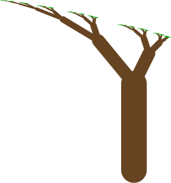
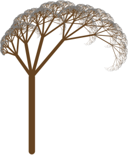
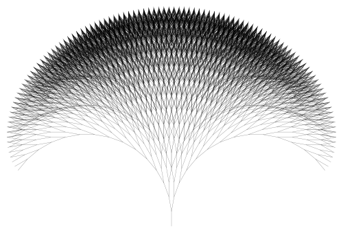
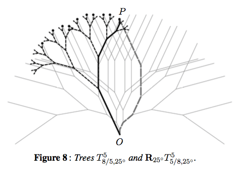
What about the case when r > 1? Let’s consider the case when r = 2 as an example. The segments in any path are of length 1, 2, 4, 8, 16, etc., getting longer each time by a power of 2. Going to a depth of n, the total length is proportional to $2^n$ in this case. In general, the total length is about $2\cdot r^n$ for arbitrary r, so scaling back by a factor of $r^n$ would keep the trees bounded as well.

So we knew how to keep the trees bounded, and started including these scaling factors when drawing our images. But there were two issues. First, we still had to do some fudging when drawing trees together with their reciprocal trees. We could still create very appealing images, but we couldn’t use the scale factor on its own.

And second — and perhaps more importantly — Nick had been doing extensive exploration on his computer generating binary trees. Right now, we had three different cases for scaling factors, depending on whether r < 1, r = 1, or r > 1. But in Nick’s experience, when he moved continuously through values of r less than 1 to values of r greater than one, the transition looked very smooth to him. There didn’t seem to be any “jump” when passing through r = 1, as happened with the scale factors we had at the moment.

I wasn’t too bothered by it, though. There are lots of instances in mathematics where 1 is some sort of boundary point. Take geometric series, for example. Or perhaps there is another boundary point which separates three fundamentally different types of solutions. For example, consider the quadratic equation

$x^2+c=0.$

The three fundamentally different solution sets correspond to c < 0, c = 0, and c > 0. There is a common example from differential equations, too, though I won’t go into that here. Suffice it to say, this type of trichotomy occurs rather frequently.

I tried explaining this to Nick, but he just wouldn’t budge. He had looked at so many binary trees, his intuition led him to firmly believe there just had to be a way to unify these scale factors.

I can still remember the afternoon — the moment — when I saw it. It was truly beautiful, and I’ll share it in just a moment. But my point is this: I was so used to seeing trichotomies in mathematics, I was just willing to live with these three scale factors. But Nick wasn’t. He was tenacious, and just insisted that there was further digging to do.

Don’t ask me to explain how I came up with it. It was like that feeling when you just were holding on to some small thing, and now you couldn’t find it. But you never left the room, so it just had to be there. So you just kept looking, not giving up until you found it.

And there is was: if the branching ratio was r and you were iterating to a depth of n, you scaled back by a factor of

$\displaystyle\sum_{k=0}^n r^k.$

This took care of all three cases at once! When r < 1, this sum is bounded (think geometric series), so the boundedness of the tree isn’t affected. When r = 1, you just get n + 1 — the same scaling factor we looked at before! And when r > 1, this sum is large enough to scale back your tree so it’s bounded.

Not only that, this scale factor made proving the Dual Tree Theorem so nice. The scaling factors for a tree with r < 1 and its reciprocal tree with branching ratio 1/r matched perfectly. No need to fudge!

This isn’t the place to go into all the mathematics, but I’d be happy to share a copy of our paper if you’re interested. We go into a lot more detail than I ever could in a blog post.

This is how mathematics happens, incidentally. It isn’t just a matter of finding a right answer, or just solving an equation. It’s a give-and-take, an exploration, a discovery here and there, tenacity, persistence. A living, breathing endeavor.

But the saga isn’t over yet…. There is a lot more to say about binary trees. I’ll do just that in my next installment of Imagifractalous!

Imagifractalous! 4: Fractal Binary Trees II

Now that the paper Nick and I wrote on binary trees was accepted for Bridges 2017 (yay!), I’d like to say a little more about what we discovered. I’ll presume you’ve already read the first Imagifractalous! post on binary trees (see Day077 for a refresher if you need it).

Recall that in that post, I discussed creating binary trees with branching ratios which were 1 or larger. Below are three examples of binary trees, with branching ratios less that 1, equal to 1, and larger than 1, respectively.

It was Nick’s insight to consider the following question: how are trees with branching ratio r related to those with branching ratio 1/r? He had done a lot of exploring with graphics in Python, and observed that there was definitely some relationship.

Let’s look at an example. The red tree is a binary tree with branching ratio r less than one, and the gray tree has a branching ratio which is the reciprocal r. Both are drawn to the same depth.

Of course you notice what’s happening — the leaves of the trees are overlapping! This was happening so frequently, it just couldn’t be coincidence. Here is another example.

tree1

Notice how three copies of the trees with branching ratio less than one are covering some of the leaves of a tree with the reciprocal ratio.

Now if you’ve ever created your own binary trees, you’ll likely have noticed that I left out a particularly important piece of information: the size of the trunks of the trees. You can imagine that if the sizes of the trunks of the r trees and the 1/r trees were not precisely related, you wouldn’t have the nice overlap.

Here is a figure taken from our paper which explains just how to find the correct relationship between the trunk sizes. It illustrates the main idea which we used to rigorously prove just about everything we observed about these reciprocal trees.

tree2

Let’s take a look at what’s happening. The thick, black tree has a branching ratio of 5/8, and a branching angle of 25°. The thick, black path going from O to P is created by following the sequence of instructions RRRLL (and so the tree is rendered to a depth of 5).

Now make a symmetric path (thick, gray, dashed) starting at P and going to O. If we start at P with the same trunk length we started with at O, and follow the exact same instructions, we have to end up back at O.

The trick is to now look at this gray path backwards, starting from O. The branches now get larger each time, by a factor of 8/5 (since they were getting smaller by a factor of 5/8 when going in the opposite direction). The size of the trunk, you can readily see, is the length of the last branch drawn in following the black path from O to P. This must be (5/8)⁵ times the length of the trunk, since the tree is of depth 5.

The sequence of instructions needed to follow this gray path is RRLLL. It turns out this is easy to predict from the geometry. Recall that beginning at P, we followed the instructions RRRLL along the gray path to get to O. When we reverse this path and go from O to P, we follow the instructions in reverse — except that in going in the reverse direction, what was previously a left turn becomes a right turn, and vice versa.

So all we need to do to get the reverse instructions is to reverse the string RRRLL to get LLRRR, and then change the L‘s to R‘s and the R‘s to L‘s, yielding RRLLL.

There’s one important detail to address: the fact that the black tree with branching ratio 5/8 is rotated by 25° to make everything work out. Again, this is easy to see from the geometry of the figure. Look at the thick gray path for a moment. Since following the instructions RRLLL means that in total, you make one more left turn than you do right turns, the last branch of the path must be oriented 25° to the left of your starting orientation (which was vertical). This tells you precisely how much you need to rotate the black tree to make the two paths have the same starting and ending points.

Of course one example does not make a proof — but in fact all the important ideas are contained in this one illustration. It is not difficult to make the argument more general, and we have successfully accomplished that (though this blog is not the place for it!).

If you look carefully at the diagram, you’ll count that there are exactly 10 leaves in common with these two trees with reciprocal branching ratios. There is some nice combinatorics going on here, which is again easy to explain from the geometry.

You can see that these common leaves (illustrated with small, black dots) are at the ends of gray branches which are oriented 25° from the vertical. Recall that this specific angle came from the fact that there was one more L than there were R‘s in the string RRLLL.

Now if you have a sequence of 5 instructions, the only way to have exactly one more L than R‘s is to have precisely three L‘s (and hence two R‘s). And the number of ways to have three L‘s in a string of length 5 is just

$\displaystyle{5\choose3}=10.$

Again, these observations are easy to generalize and prove rigorously.

And where does this take us?

On the right are 12 copies of a tree with a braching ratio of r less than one and a branching angle of 30°, and on the left are 12 copies of a tree with a reciprocal branching ratio of 1/r, also with a branching angle of 30°. All are drawn to depth 4, and the trunks are appropriately scaled as previously discussed.

These sets of trees produce exactly the same leaves! We called this the Dual Tree Theorem, which was the culmination of all these observations. Here is an illustration with both sets of trees on top of each other.

As intriguing as this discovery was, it was only the beginning of a much broader and deeper exploration into the fractal world of binary trees. I’ll continue a discussion of our adventures in the next installment of Imagifractalous!