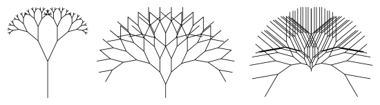
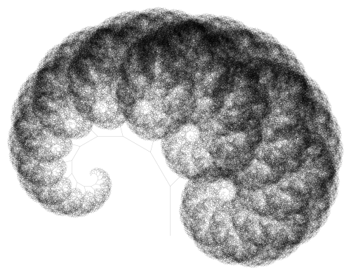
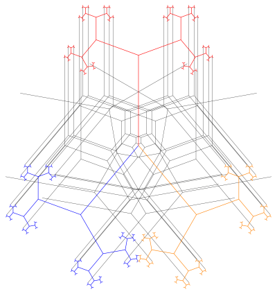
A few weeks, ago I dug out a problem which had puzzled me for over three years. I finally decided that now it was time to really dig in — and to my surprise and delight, not only did I solve the problem, but I’ve already got a draft of a paper written! The figure below is from that paper.

The problem is yet another variation on the recursion which produces the Koch snowflake. I discussed the Koch snowflake in one my first posts, so visit my Day007 post on this fascinating fractal for a refresher.
So what is the variation here? Consider the general recursive scheme

where 

The Koch curve is generated by choosing

Previously I’ve studied cases where 

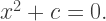
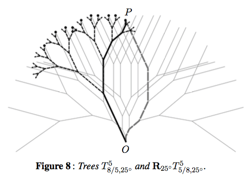
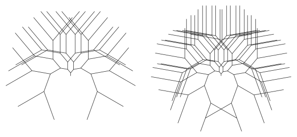
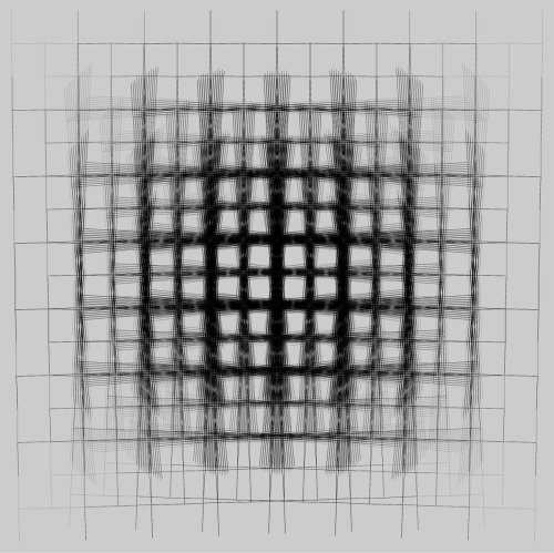
So let’s investigate the example illustrated above in more detail. The recursive scheme which generates this spiral is given by

How does this scheme draw a spiral arm? Let’s look at the figure below.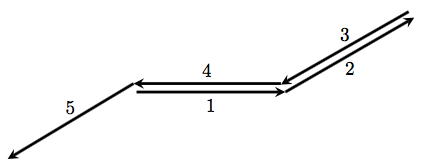
We begin at the origin, and then draw a segment at 


The next turn is 

What next? It is at this point that we invoke a recursive call — and so the next angle tells us what direction the next arm will be drawn in. Of course, like before, the three angles after that will continue drawing the arm and then bring us back to the origin, awaiting the next recursive call.
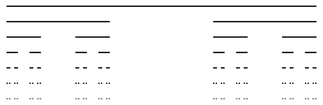
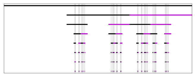
This behavior can be illustrated in the following chart.
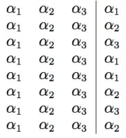
Here, the angles turned are listed in rows of four, one after another. The first three angles in each row are the same, and their job is to complete the arm once a direction is chosen. But the direction chosen is determined by the fourth column (separated by the divider), whose behavior is not periodic and highly recursive.
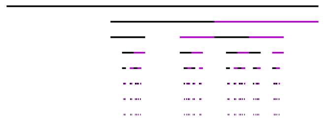
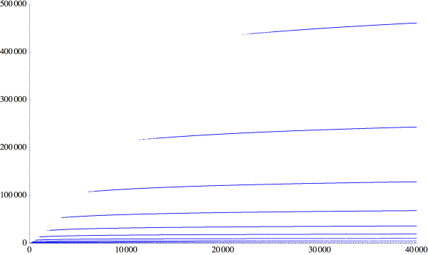
So where do we go from here? The next chart we’ll look it is a chart of the directions the arms are drawn in.
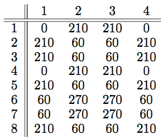
We read this chart in rows as follows: the first arm is drawn at an angle of 
But the third arm exactly retraces the second arm drawn, since it is pointed in the direction of 

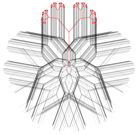
So you can see what’s going on. One important consequence of the recursive algorithm is that the arms keep being retraced over and over again.
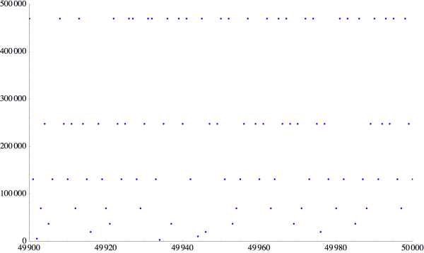
When will the complete spiral be drawn? Well, we need to see every multiple of
How would you show this? We can’t go into all the details here. The important observation is that if you read across the chart one row at a time, you get the same sequence of angles by reading down the first column of the chart.
But it isn’t enough to just observe this — it has to be proved. This is where some elementary number theory comes in. No more than what might be seen in an undergraduate number theory course, but beyond the scope of this post.
Slight step up on my soapbox — while I usually deplore the definition of mathematics as the “science of finding patterns” (as this only scratches the surface), in this case, finding patterns is critically important. With some trial and error, you hit upon making charts in rows of four, and then putting the directions the arms are drawn in rows of four, and then stare at the numbers until you notice patterns in the charts. The trick is knowing what to prove — once stated properly, the results almost prove themselves.
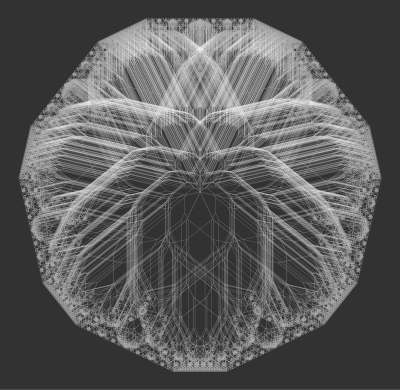
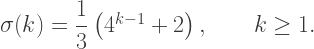
You’ll have to wait for the paper to come out for all the details. But here is a brief summary. Suppose you divide the circle into n parts, where n is even. Then devise a recursive scheme using the turning angles

Now define
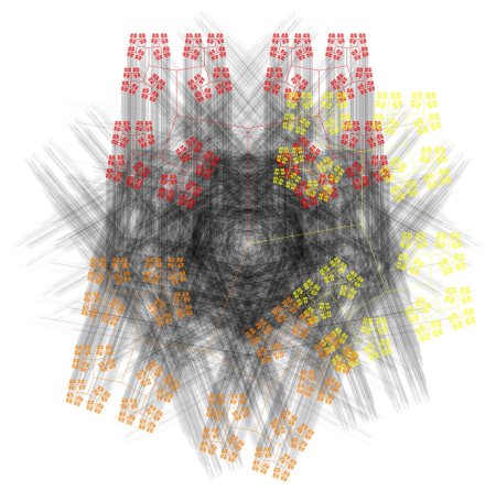
When n is divisible by 4, the spiral has n arms, and you need to draw exactly 
But when n is even but not divisible by four, the spiral only has n/2 arms, and it takes 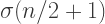
Absolutely amazing, in my opinion. I formulated these conjectures over three years ago, but got stuck. A few weeks ago I had the house to myself for a while, and I just sat down and said to myself, “Look, you’ve already written one paper on these recursions. You can do this.”
And within two days, I worked out the patterns. Then the proofs, and within a week, a draft of the paper.
I am always humbled by such a seemingly innocuous problem — generating a simple spiral . But there are so many levels to this problem, and so much interesting mathematics to be discovered. I’ll continue exploring recursively drawn images, and share the amazing results with you when I find them!

 for example.
 Conjecture: Suppose
  and
and  are given. Then using the factorial function and the function
 and
and  from
from  and so on, but you’ve got to get larger first, and that requires some use of the factorial.
 there exist positive integers
  such that
 is composed
  times.
 The Possibility Lemma is only a starting point, since it turns out that most of the time, the smallest
  need to generate a particular
  is actually greater than
  the smallest
  with
with  so that
 we get

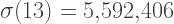
 is
is  and computations with such large factorials take time. It turns out that the trick was to compute in advance the first 1,000,000 factorials as floating point numbers. A little accuracy is lost as result, but several checks suggested that even so, the correct value of
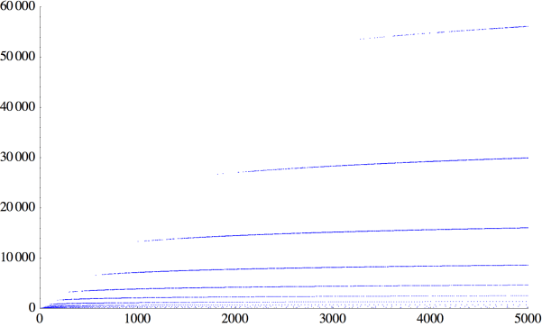
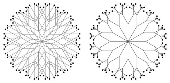
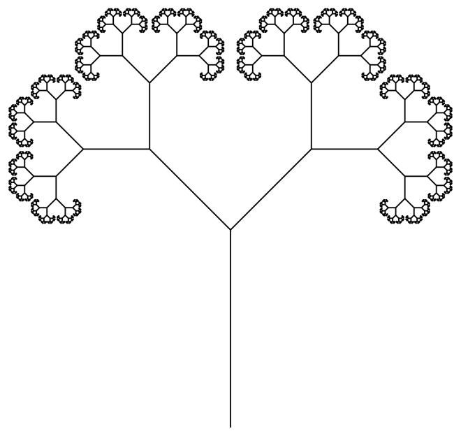
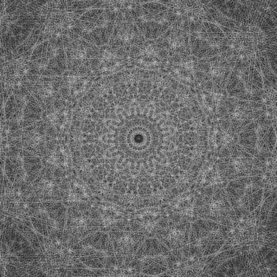
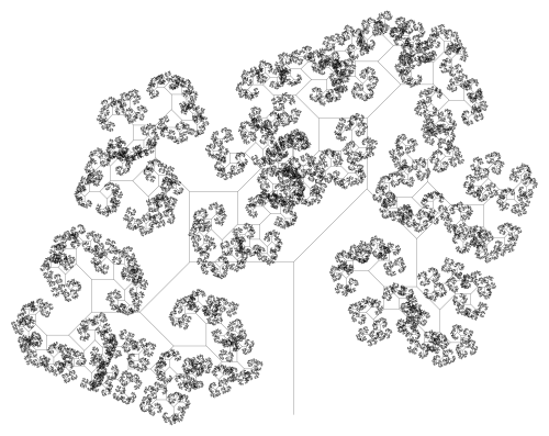
 generates the following graph, so it seems that there may be similar behavior for various
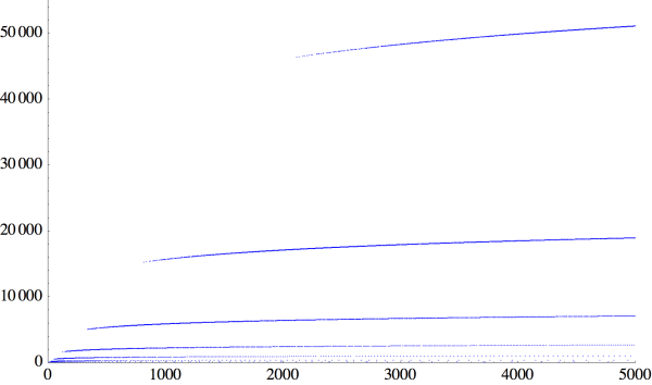


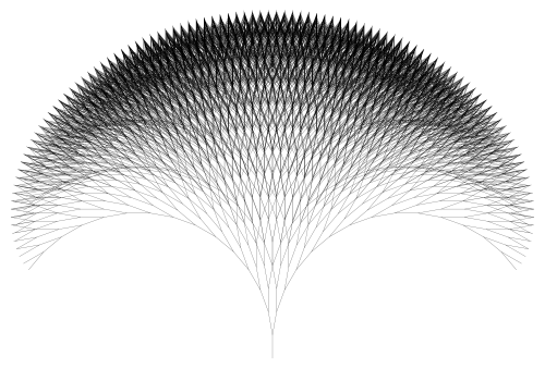
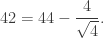
 in this case. In general, the total length is about
  for arbitrary r, so scaling back by a factor of
  would keep the trees bounded as well.