Imagifractalous! 3: Fractal Binary Trees

I’ve taken a break from Koch-like curves and p-adic sequences for an arboreal interlude….  Yes, there’s a story about why — I needed to work with Nick on a paper he was writing for Bridges — but that story isn’t quite finished yet.  When it is, I’ll tell it.  But for now, I thought I’d share some of the fascinating images we created along the way.

Let’s start with a few examples of simple binary trees.  If you want to see more, just do a quick online search — there are lots of fractal trees out there on the web!  The construction is pretty straightforward.  Start by drawing a vertical trunk of length 1.  Then, move left and right some specified angle, and draw a branch of some length r < 1.  Recursively repeat from where you left off, always adding two more smaller branches at the tip of each branch you’ve already drawn.

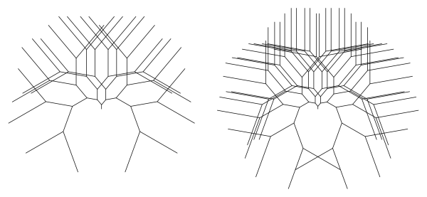
If you look at these two examples for a moment, you’ll get the idea.  Here, the angle used is 40 degrees, and the ratio is 5/8.  On the left, there are 5 iterations of the recursive drawing, and there are 6 iterations on the right.

Here’s another example with a lot more interaction among the branches.

This type of fractal binary tree has been studied quite a bit.  There is a well-known paper by Mandelbrot and Frame which discusses these trees, but it’s not available without paying for it.  So here is a paper by Pons which addresses the same issues, but is available online.  It’s an interesting read, but be forewarned that there’s a lot of mathematics in it!

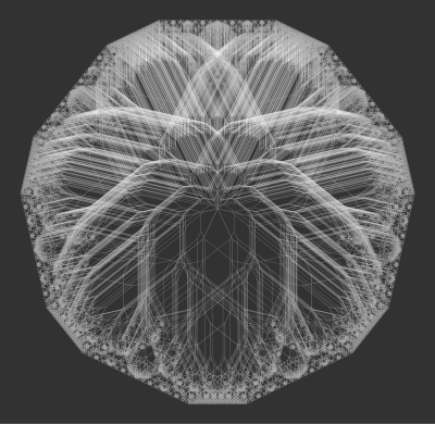
In trying to understand various properties of these fractal trees, it’s natural to write code which creates them.  But here’s the interesting thing about writing programs like that — once they’re written, you can input anything you like!  Who says that r has to be less than 1?  The tree above is a nice example of a fractal tree with r = 1.  All the branches are of the same length, and there is a lot of overlap.  This helps create an interesting texture.

But here’s the catch.  The more iterations you go, the bigger the tree gets.  In a mathematical sense, the iterations are said to be unbounded.  But when Mathematica outputs a graphic, it is automatically scaled to fit your viewing window.  So in practice, you don’t really care how large the tree gets, since it will automatically be scaled down so the entire tree is visible.

It is important to note that when r < 1, the trees are bounded, so they are easier to study mathematically.  The paper Nick and I are working on scales unbounded trees so they are more accessible, but as I said, I’ll talk more about this in a later post.

Here are a few examples with r > 1.  Notice that as there are more and more iterations, the branches keep getting larger.  This creates a very different type of binary tree, and again, a tree which keeps getting bigger (and unbounded) as the number of iterations increases.  But as mentioned earlier, Mathematica will automatically scale an image, so these trees are easy to generate and look at.

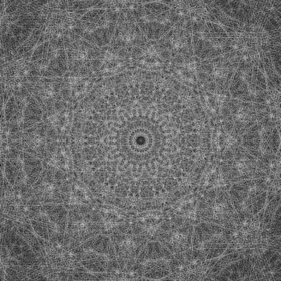
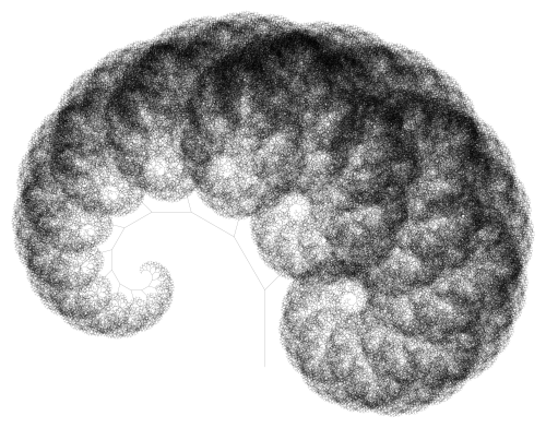
Nick created the following image using copies of binary trees with r approximately equal to 1.04.  The ever-expanding branches allow for the creation of interesting textures you really can’t achieve when r < 1.

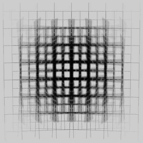
Another of my favorites is the following tree, created with r = 1.  The angle used, though, is 90.9 degrees.  Making the angle just slightly larger than a right angle creates an interesting visual effect.

But the exploration didn’t stop with just varying r so it could take on values 1 or greater.  I started thinking about other ways to alter the parameters used to create fractal binary trees.

For example, why does r have to stay the same at each iteration?  Well, it doesn’t!  The following image was created using values of r which alternate between iterations.

And the values of r can vary in other ways from iteration to iteration.  There is a lot more to investigate, such as generating a binary tree from any sequence of r values.  But studying these mathematically may be somewhat more difficult….

Now in a typical binary tree, the angle you branch to the left is the same as the angle you branch to the right.  Of course these two angles don’t have to be the same.  What happens if the branching angle to the left is different from the branching angle to the right?  Below is one possibility.

And for another possibility?  What if you choose two different angles, but have the computer randomly decide which is used to branch left/right at each iteration?  What then?

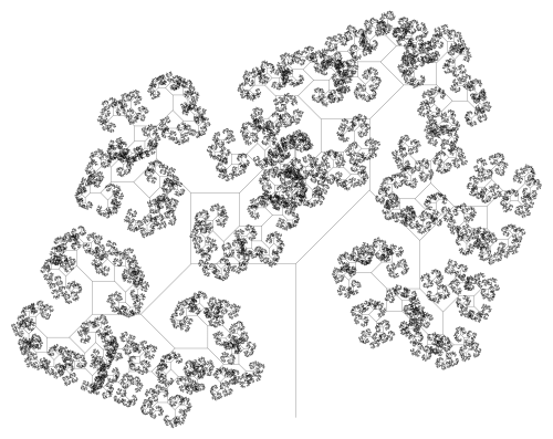
Here is one example, where the branching angles are 45 and 90 degrees, but which is left or right is chosen randomly (with equal probability) at each iteration.  Gives the fractal tree a funky feel….

You might have noticed that none of these images are in color.  One very practial reason is that for writing Bridges papers, you need to make sure your images look OK printed in black-and-white, since the book of conference papers is not printed in color.

But there’s another reason I didn’t include color images in this post.  Yes, I’ve got plenty…and I will share them with you later.  What I want to communicate is the amazing variety of textures available by using a simple algorithm to create binary trees.  Nick and I never imagined there would be such a fantastic range of images we could create.  But there are.  You’ve just seen them.

Once the Bridges paper is submitted, accepted (hopefully!), and revised, I’ll continue the story of our arboreal adventure.  There is a lot more to share, and it will certainly be worth the wait!