April 2016 – Creativity in Mathematics

Creating Fractals VIII: PostScript Programming

June 1998.

That’s when I wrote the code I’m going to talk about today.

When I became interested in computer graphics, a windows environment you’re used to by now just didn’t exist. For example, the computer I used (called a Zenith H19) had a screen 80 x 25 characaters. Yes, characters. Rather like a larger version of those still unimaginable TI calculator screens (couldn’t resist).

There was no graphical user interface (GUI), mouse, touch-screen. If you wanted to draw a picture, you had to write a computer program to do it.

And if you wanted to see what it looked like, well, you had to print it out.

Yep. That was the only way to see if your code was correct. It made debugging very challenging. But that’s all there was. So I learned how to write PostScript code.

There are two features of PostScript I want to discuss today. First, the syntax is written in postfix notation, like most HP calculators. If you wanted to add 2 and 3 on a typical calculator, you’d type in “2 + 3 =.” The result would be 5. This is called infix notation, where the operator is written in between the arguments.

In PostScript, though, you’d write “2 3 add.” In other words, the arguments come first. Then they’re added together — the operator comes last, which is referred to as postfix notation. So if you wanted to write

(2 + 3 ) x (10 – 4)

in PostScript, you’d write

2 3 add 10 4 sub mul.

Notice that the multiplication is done last.

When programming in Python, most functions are described using prefix notation. In other words, you give the function name first, and then the arguments to the function. For example, randint(1,10) would output a random number between 1 and 10, inclusive. If we had to write the arithmetic expression above in prefix notation, it would look like

times(add(2,3), subtract(10,4)).

You probably encounter these ideas on a daily basis. For example, if you want to delete a bunch of files, you first select them, and then do something like click “Move to trash” from a dropdown menu. But if you’re writing an email, you usually click on the attach icon first, and then select the files you’d like to attach. Postfix and prefix.

Of course this is just an introduction to using the different types of notation. In general, you’d transform the above arithmetic expression into what it called an expression tree, like this: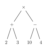 expressiontree

Then prefix notation may be derived from a preorder traversal of the expression tree, infix notation from an inorder traversal of the tree, and finally, postfix notation comes from a postorder traversal of the tree. Feel free to ask the internet all about binary trees and tree traversals. Trees are very important data structures in computer science.

The second feature of PostScript I’d like to discuss today is that it is an example of a stack-based language. For example, if you typed

4 5 3 7 8

in a PostScript program, the number 4 would be pushed onto the stack — that is, the working memory of the program — and then 5, then 3, 7, and finally 8. (For convenience, we’ll always think of the bottom of the stack as being on the left, and the top of the stack as being on the right. Easier to write and read that way.)

If you want to follow along, do the following: write 4 on an index card or small piece of paper, then write 5 on another and put it on top of the 4, and so on, until you put the 8 on top of the stack. You really do have a stack of numbers.

Now when you type the “add” function, PostScript thinks, “OK, time to add! What are the top two numbers on the stack? Oh, 8 and 7! I’ll add these and put the sum back on the stack for you!”

So you type

4 5 3 7 8 add,

and PostScript performs the appropriate action and the stack now becomes

4 5 3 15.

If you now want to divide (div in PostScript), the interpreter looks at the top number on the stack and divides it by the second number on the stack, and puts that result on the stack. So

4 5 3 7 8 add div

would create the stack

4 5 5.

You should be able to figure out that

4 5 3 7 8 add div mul sub

would just leave the single number 21 on the stack.

Graphics are drawn this way, too. For example, we would create a square with the commands

0 0 moveto 0 1 lineto 1 1 lineto 1 0 lineto 0 0 lineto closepath stroke.

Again, the arguments come first. We move to the point (0,0), and then draw a line segment to (0,1), and so forth. Closepath “ties” the beginning and end of our path together, and the command “stroke” actually draws the square on the page.

Commands like

1 0.5 0 setrgbcolor

set the current color to orange, and

5 setlinewidth

sets the width of lines to be drawn. You can change any aspect of any drawn image — the only limit is your imagination!

Of course this is only the most basic introduction to the PostScript programming language. But if you’re interested, there’s good news. First, it shouldn’t be hard to download a PostScript interpreted for your computer. I use MacGhostView — installing will also require you to install XQuartz, too, but not to worry.

Second, there are some great resources online. Back when I was learning PostScript, there were three very helpful books — the Blue Book, the Red Book, and the Green Book. Yep, that’s what there were called. The Blue Book is the place you should start — it includes a tutoral on all the basics. The Red Book is the Reference Manual — handy in that it lists PostScript commands, their syntax, and examples of how to use them. The Green Book is for the serious programmer, and discusses at a high level how the PostScript language is organized.

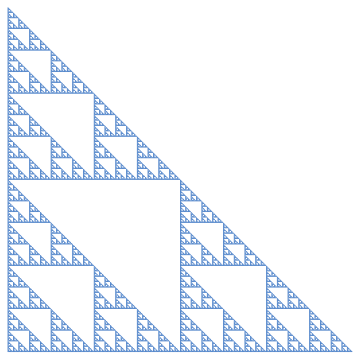
Finally, here is the code I wrote all those years ago! (Click here: Sierpinski.) I did modify the original code so it produces a Sierpinski triangle. It will be a little daunting to figure out if you’re just starting to learn PostScript, but I include it as it motivated me to talk about PostScript today.

And a final few words about motivation. Try to learn programming languages which expose you to different ways of thinking. This develops flexibility of mind for coding in general. Whenever I learn a new language, I’m always thinking things like, “Oh, that’s the same as stacks in PostScript,” or “Yeah, like maps in LISP.”

As you learn more, your programming toolbox gets bigger, and you find that the time it takes from conceiving of an idea to successfully implementing it becomes shorter and shorter. That’s when it starts really getting fun….

Creating Fractals VII: Iterated Function Systems III

Today, we’re going to wrap up our discussion of iterated function systems by looking at an algorithm which may be used to generate fractal images.

Recall (look back at the first post if you need to!) the Sierpinski triangle. No matter what initial shape we started with, the iterations of the function system eventually looked like the Sierpinski triangle.

Sierp4

But there’s a computational issue at play. Since there are three different transformations, each iteration produces three times the number of objects. So if we carried out 10 iterations, we’d have 3¹⁰ = 59,049 objects to keep track of. Not too difficult for a computer.

But let’s look at the Sierpinski carpet. With eight different transformations, we’d have 8¹⁰ = 1,073,741,824 objects to keep track of. Keeping track of a billion objects just isn’t practical.

Of course you could use fewer iterations — but it turns out there’s a nice way out of this predicament. We can approximate the fractal using a random algorithm in the following way.

Begin with a single point (usually (0,0) is the easiest). Then randomly choose a function in the system, and apply it to this point. Then iterate: keep randomly choosing a function from the system, then apply it to the last computed point.

What the theory says (again, read the Barnsley book for all the proofs!) is that these points keep getting closer and closer to the fractal image determined by the system. Maybe the first few are a little off — but if we just get rid of the first 10 or 100, say, and plot the rest of the points, we can get a good approximation to the fractal image.

Consider the Sierpinski triangle again. Below is what the first 20 points look like (after (0,0)), numbered in the order in which they’re produced.

Let’s look at this in a bit more detail. For reference, we’ll copy the function system which produces the Sierpinski triangle from the first post.

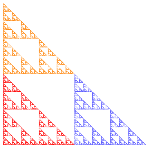
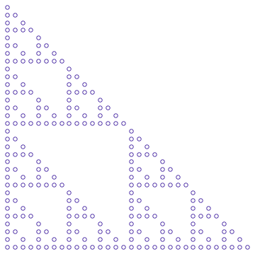
$F_1\left(\begin{matrix}x\\y\end{matrix}\right)=\left[\begin{matrix}0.5&0\\0&0.5\end{matrix}\right] \left(\begin{matrix}x\\y\end{matrix}\right)$

$F_2\left(\begin{matrix}x\\y\end{matrix}\right)=\left[\begin{matrix}0.5&0\\0&0.5\end{matrix}\right] \left(\begin{matrix}x\\y\end{matrix}\right)+\left(\begin{matrix}1\\0\end{matrix}\right)$

$F_3\left(\begin{matrix}x\\y\end{matrix}\right)=\left[\begin{matrix}0.5&0\\0&0.5\end{matrix}\right] \left(\begin{matrix}x\\y\end{matrix}\right)+\left(\begin{matrix}0\\1\end{matrix}\right)$

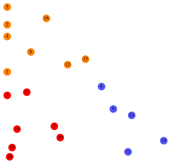
Now here’s how the color scheme works. Any time $F_1$ is randomly chosen, the point is colored red. For example, you can see that after Point 6 was drawn, $F_1$ was chosen, so Point 7 was simply halfway between Point 6 and the origin.

Any time $F_2$ is chosen, the point is colored blue. For example, after Point 8 was drawn, $F_2$ was randomly chosen. You can see that if you move Point 8 halfway to the origin and then over right one unit, you land up exactly at Point 9.

Finally, any time $F_3$ is chosen, the point is colored orange. So for example, it should be clear that moving Point 7 halfway toward the origin and then up one unit results in Point 8.

Of course plotting more points results in a more accurate representation of the fractal. Below is an image produced using 5000 points.

To get more accuracy, simply increase the number of points, but decrease the size of the points (so they don’t overlap). The following image is the result of increasing the number of points to 50,000, but using points of half the radius.

Sierp50000

There’s just one more consideration, and then we can move on to the Python code for the algorithm. How do we randomly choose the next affine transformation?

Of course we use a random number generator to select a transformation. In the case of the Sierpinski triangle, each of the three transformations had the same likelihood of being selected.

Now consider one of the fractals we looked at last week.

Two4

If the algorithm chose either transformation with equal probability, this is what our image would look like:

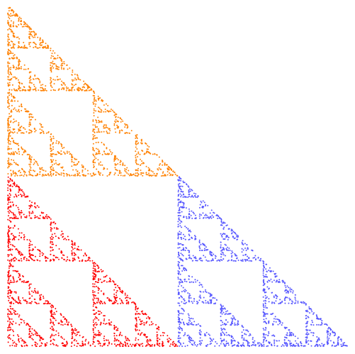
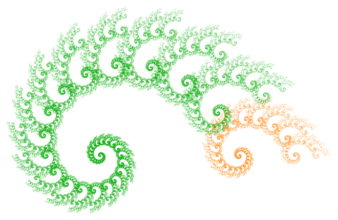
Of course there’s a huge difference! What’s happening is that transformation $F_{{\rm orange}}$ actually corresponds to a much smaller portion of the fractal than $F_{{\rm green}}$ — and so to get a more realistic idea of what the fractal is really like, we need to choose it less often. Otherwise, we overemphasize those parts of the fractal corresponding to the effect of $F_{{\rm orange}}.$

Again, according to the theory, it’s best to choose probabilities roughly in proportion to the portions of the fractal corresponding to the affine transformations. So rather than a 50/50 split, I chose $F_{{\rm green}}$ 87.5% of the time, and $F_{{\rm orange}}$ just 12.5% of the time. As you’ll see when you experiment, a few percentage points may really impact the appearance of a fractal image.

From a theoretical perspective, it actually doesn’t matter what the probabilities are — if you let the number of points you draw go to infinity, you’ll always get the same fractal image! But of course we are limited to a finite number of points, and so the probabilities do in fact strongly influence the final appearance of the image.

So once you’ve chosen some transformations, that’s just the beginning. You’ve got to decide on a color scheme, the number of points and their size, as well as the probabilities that each transformation is chosen. All these choices impact the result.

Now it’s your turn! Here is the Sage link to the python code which you can use to generate your own fractal images. (Remember, you’ve got to copy it into one of your own Projects first.) Freely experiment — I’ve also added examples of non-affine transformations, as well as affine transformations in three dimensions!

And please comment with interesting images you create. I’m interested to see what you can come up with!

Creating Fractals VI: Iterated Function Systems II

What I find truly remarkable about iterated function systems is the astonishing variety of fractals you can create with just two affine transformations. Today, we’ll explore some more examples so you can get a better feel for how the particular affine transformations used affect the final image.

Let’s begin with the example from last week, which I color coded for easy reference.

Below are the affine transformations which generated this fractal.

$F_{{\rm green}}\left(\begin{matrix}x\\y\end{matrix}\right)=\left[\begin{matrix}0.95&0\\0&0.95\end{matrix}\right]\left[\begin{matrix}\cos(20^\circ)&-\sin(20^\circ)\\\sin(20^\circ)&\cos(20^\circ)\end{matrix}\right]\left(\begin{matrix}x\\y\end{matrix}\right)$

$F_{{\rm orange}}\left(\begin{matrix}x\\y\end{matrix}\right)=\left[\begin{matrix}0.4&0\\0&0.4\end{matrix}\right]\left(\begin{matrix}x\\y\end{matrix}\right)+\left(\begin{matrix}1\\0\end{matrix}\right)$

Now compare the different colors in the image with the transformations. The first transformation combines a scaling by 0.95 with a rotation by 20 degrees. If you look closely, you’ll see that the green part of the image looks the same as a slightly smaller copy of the entire fractal, except rotated by 20 degrees from the center of the spiral (note that there is no translation involved in $F_{{\rm green}}$ ).

The orange part of the image is simply a scaled version of the entire fractal (by a factor of 0.4), but moved over 1 unit. You can see this by looking at the form of the affine transformation $F_{{\rm orange}}.$

The pair of affine transformations used to generate the spiral exactly describes the self-similarity. This is easy to see after the fact — but I really have no helpful suggestion as to how to predict the form of this wonderful spiral just by looking at the transformations.

Now let’s just slightly alter the second transformation so that in addition to scaling by a factor of 0.4, there is a shear as well.

$F_{{\rm orange}}\left(\begin{matrix}x\\y\end{matrix}\right)=\left[\begin{matrix}0.4&0.4\\0&0.4\end{matrix}\right]\left(\begin{matrix}x\\y\end{matrix}\right)+\left(\begin{matrix}1\\0\end{matrix}\right)$

Notice how the fractal changes.

The shear distorts each arm of the spiral — stretching it in the process and creating more interaction between the various arms.

Now let’s go back to the original spiral and change the first transformation instead, slightly altering the scale factor.

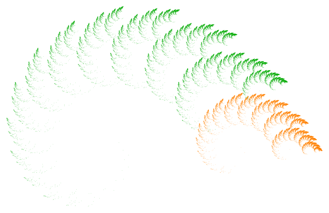
$F_{{\rm green}}\left(\begin{matrix}x\\y\end{matrix}\right)=\left[\begin{matrix}0.9&0\\0&0.9\end{matrix}\right]\left[\begin{matrix}\cos(20^\circ)&-\sin(20^\circ)\\\sin(20^\circ)&\cos(20^\circ)\end{matrix}\right]\left(\begin{matrix}x\\y\end{matrix}\right)$

Here is what happens:

Two4

I really don’t how to predict that this is what would happen — but I find it fascinating how even small changes in parameters can really change the way a fractal looks.

I can’t resist one more image created by changing the second transformation to

$F_{{\rm orange}}\left(\begin{matrix}x\\y\end{matrix}\right)=\left[\begin{matrix}0.4&0\\0.4&0.15\end{matrix}\right]\left(\begin{matrix}x\\y\end{matrix}\right)+\left(\begin{matrix}1\\0\end{matrix}\right).$

Here is the result.There’s so much you can do with just one pair of transformations!

While it may not be possible to guess exactly what a fractal will look like, it’s possible to know some features of a fractal based upon how you set up your transformations. For example, condsider this combination of a shear and a scaling:

$G_1\left(\begin{matrix}x\\y\end{matrix}\right)=\dfrac23\left[\begin{matrix}1&-1/2\\0&1\end{matrix}\right]\left(\begin{matrix}x\\y\end{matrix}\right)+\left(\begin{matrix}1\\1\end{matrix}\right).$

There will be some aspect of the fractal which can be described by a shear. For the second transformation, just take the opposite of the first, as follows.

$G_2\left(\begin{matrix}x\\y\end{matrix}\right)=-\dfrac23\left[\begin{matrix}1&-1/2\\0&1\end{matrix}\right]\left(\begin{matrix}x\\y\end{matrix}\right)-\left(\begin{matrix}1\\1\end{matrix}\right).$

This must force the fractal to have 180 degree rotational symmetry! Think about how the algorithm works — take the image under one transformation, then the other — but by their definitions, the images must be symmetric about the origin.

So it is possible to use our knowledge of affine transformations to design, even if to a limited extent, some features of the resulting fractal.

As another example, we can assemble a fractal similar to two smaller copies of itself, one piece of which is a 90 degree rotation of the other. Use $G_1$ as above, and then use

$G_2=\left[\begin{matrix}0&-1\\1&0\end{matrix}\right]G_1.$

Here is the resulting fractal.

You can clearly see how the red piece is a 90 degree counterclockwise rotation of the purple piece. This follows from how we created the second transformation from the first.

One reason for the diversity of fractals is the number of parameters needed to specify two affine parameterizations — twelve in all. Now some sets of parameters may create the same fractal — but even so, the wealth of variations is still staggering.

But will just any affine transformations work? There are some constraints — for example, you can’t describe a fractal in terms of larger copies of itself. So the affine transformations cannot make a starting object bigger, or else each successive iteration will expand. Of course you can still use such affine transformations to create interesting graphical effects — but the resulting image will not be an approximation to a fractal.

Next week, we’ll look at the algorithm which I used to create all these fractal images, and I’ll give you some Python code you can use yourself. But before I close, I’d like to share a few favorite fractals which are generated by just two affine transformations.

First, the Beetle. It looks like it’s scampering toward you.

And the second, well, it’s just yellow.

Until next week!

Creating Fractals V: Iterated Function Systems I

So just what are fractals?

In this blog, we’ve looked at a few examples of fractals so far — the Koch snowflake, for example — and informally called images created by the same algorithm “fractal images.” But what makes the Koch snowflake a fractal?

Regardless of which definition you find on the internet, you’ll find ideas about self-similarity which keeps being repeated at ever smaller scales. Truly rigorous definitions require some truly advanced mathematics…but we’ll illustrate the idea with another classic fractal, the Sierpinski triangle.

Begin with any triangle, and then remove the triangle formed by connecting the midpoints of the sides, as shown below.

Sierp1

Now repeat — in each triangle, remove the triangle formed by connecting the midpoints of the sides. Two more iterations results in the following image.

And five more iterations gives the Sierpinski triangle.

Sierp3

Of course, in a mathematical sense, this process goes on infinitely — you still keep getting triangles on each iteration, so you’re never done. But as far as creating computer graphics is concerned, you can just stop when the iterations start looking the same.

The self-similarity of the Sierpinski triangle should now be fairly evident. The way it’s constructed, you’ll notice that each of the three smaller triangles shown in the first iteration looks identical to the entire Sierpinski triangle, except that it’s shrunk by a factor of two along all dimensions. This is self-similarity: one can say that the Sierpinski triangle is, in a mathematical sense, built up of smaller copies of itself.

Now how can we describe this self-similarity? Using affine transformations. (If the notations and functions below aren’t familiar to you, study up on linear and affine transformations, and how you use matrices to represent them.)

First, we’ll color code parts of the Sierpinski triangle for easy reference.

Next, we’ll introduce a coordinate system. Let the origin be the vertex of the right angle of the triangle, with the usual x– and y-axes. If you apply the transformation

$F_1\left(\begin{matrix}x\\y\end{matrix}\right)=\left[\begin{matrix}0.5&0\\0&0.5\end{matrix}\right] \left(\begin{matrix}x\\y\end{matrix}\right)$

to the entire Sierpinski triangle, you get the red “shrunk by half” triangle at the right angle of the Sierpinski triangle.

Now if you apply the transformation

$F_2\left(\begin{matrix}x\\y\end{matrix}\right)=\left[\begin{matrix}0.5&0\\0&0.5\end{matrix}\right] \left(\begin{matrix}x\\y\end{matrix}\right)+\left(\begin{matrix}1\\0\end{matrix}\right)$

to the Sierpinski triangle, you’ll get the blue portion — shrunk by a factor of two, and moved over one unit. Finally, if you apply the transformation

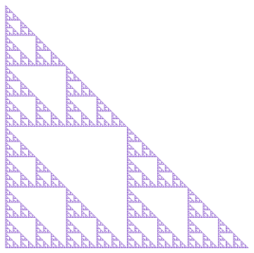
$F_3\left(\begin{matrix}x\\y\end{matrix}\right)=\left[\begin{matrix}0.5&0\\0&0.5\end{matrix}\right] \left(\begin{matrix}x\\y\end{matrix}\right)+\left(\begin{matrix}0\\1\end{matrix}\right),$

you’ll get the orange part, shrunk by a factor of two and moved up one unit. (Note that the choice of moving one unit is arbitrary — you’ll get something that looks like the Sierpinski triangle as long as you move the same amount in each direction.)

What all this means is that the functions $F_1,$ $F_2,$ and $F_3$ mathematically describe the self-similarity of the Sierpinski triangle, and so they may be used to generate the Sierpinski triangle. You can see where the term iterated function system comes from by thinking about using these functions iteratively to generate a fractal image.

Now here’s the amazing part. If you look at the very first iteration we did, you’ll see three triangles, each representing one of these transformations. So imagine beginning with a different object — say a unit square — and perform these three transformations; that is, shrink by half, shrink and move to the right, and shrink and move up. You’ll get something like this:

Sierp21

After two more iterations, here is what you’ll see.

Sierp22

Notice the self-similarity. If we keep going another six iterations, we get…

Sierp23

…the Sierpinski triangle again!

If you start out with a small circle, you get the following after five iterations.

Sierp31

What this means is that the Sierpinski triangle — in a very real, rigorously mathematical sense — is completely determined by the transformations which describe its self-similarity. Yes, the final result is always a triangle, independent of what shape you start out with! Filled squares, circles, whatever object you choose — the result will always be the Sierpinski triangle.

If you really want to know why, read Michael Barnsley’s Fractals Everywhere. But be forewarned — you need to know a lot of mathematics to completely understand what’s going on. But it really is amazing.

In order to create your own fractals, you don’t need to know all the mathematical details. You just need to understand the nature of self-similarity, and how to represent it using affine transformations.

Another famous fractal is the Sierpinski carpet.

Carpet

You can see the self-similarity here as well. Note that there are eight smaller, identical copies of the Sierpinski carpet which make up the fractal. So you would need eight affine transformations, one of which would be

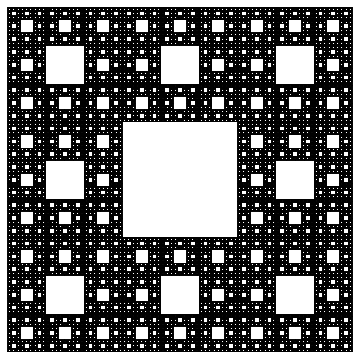
$G\left(\begin{matrix}x\\y\end{matrix}\right)=\left[\begin{matrix}1/3&0\\0&1/3\end{matrix}\right] \left(\begin{matrix}x\\y\end{matrix}\right)+\left(\begin{matrix}1\\0\end{matrix}\right).$

Notice that the scaling is only by a factor of $1/3$ here, and that the choice of units to move is arbitrary (as with the Sierpinski triangle). Further, it doesn’t matter what object you begin with — you’ll always end up with the Sierpinski carpet when your done.

Where do we go from here? Next week, we’ll look at how different choices of affine transformations affect the fractal image. For example, suppose we return to the Sierpinski triangle example, but replace $F_1$ with the transformation

$F_1\left(\begin{matrix}x\\y\end{matrix}\right)=\left[\begin{matrix}0.25&0\\0&0.5\end{matrix}\right] \left(\begin{matrix}x\\y\end{matrix}\right).$

How should this affect the fractal? Look at the result, and see if you can figure it out.

NewSierp

Can you see the two identical copies, each shrunk by half, generated by $F_2$ and $F_3$ ? But note that the copy at the right angle is actually shrunk by one-fourth along the x direction — but this is expected as a result of the scaling by $0.25$ along the x direction in $F_1.$

In other words, when we change the description of the self-similarity (that is, when we change the affine transformations), we change what the fractal looks like — because, in a mathematical sense, the fractal is the set of affine transformations. But here’s the difficult question — can you predict what the fractal will look like only by looking at the affine transformations?

Well, if you can, then you’re a lot better at this than I am! It’s not an easy task — but it is what makes creating fractals fun. Usually, you don’t know what the result will be. That’s the adventure! You often surprise yourself by what you discover.

In the next few posts, we’ll consider different types of affine transformations (like rotations, shears, etc.), and then discuss an algorithm which can generate approximations to fractals. Stay tuned!

P.S. This fractal was created using only two affine transformations. Next week we’ll see how.