September 2017 – Creativity in Mathematics

Mathematics and Digital Art: Update 1 (Fall 2017)

About a month has passed since beginning my third semester of Mathematics and Digital Art! As with last semester, I plan on giving updates about once a month to discuss changes in the course and to showcase student work.

The main difference this semester (as I discussed a few weeks ago) was starting with Processing right from the beginning. From my perspective, the course has run more smoothly than ever — and some of my students are already really getting into the coding aspect of creating digital art.

I do believe that beginning this way will pay off when we get to making movies. Since we’ll already know the basics and understand the difference between user space and screen space, I can focus more on the interactive abilities of Processing — such as having features of the displayed image change by moving the mouse or pressing different keys on the keyboard.

The first two assignments were essentially the same as last semester. We began with discussing color and the work of Josef Albers, emphasizing the fact that there is no such thing as “pure color” — colors are only perceived in relation to other colors.

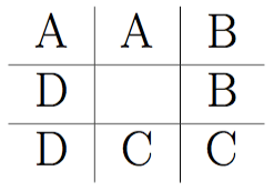
Again, I was surprised by the diversity of the images students created. Like last year, a few students experimented with a minimalist approach. Here is what Alex generated using just a 2-by-2 grid of squares.

Day112Alex

I should point out that outlining the geometrical objects (using the strokeWeight function) is not “pure” Albers — you aren’t really seeing one color on top of another due to the black outlines. But I did have students submit three pieces, insisting that one of the pieces was created only by changing the parameters in the original Albers routine, as shown in the following submission.

Day112Linh2

Here is Courtney’s submission on this theme, again created only by changing parameters to the drawing routine.

Day112Courtney

Most students — I think in part due to the fact that we started discussing code even earlier than previous semesters — really pushed the geometry far beyond the simple idea of rectangles within rectangles.

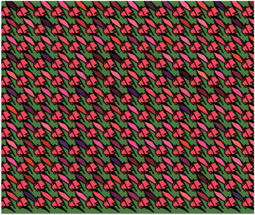
While toying with various geometrical motifs, Tera found something that reminded her of a rose. This influenced her color palette: reds and pinks for the flowers, with a green background, meant to suggest that the flowers were in a garden.

Day112Tera

Cissy explored the geometry as well. Note how keeping the stroke weight at zero — so that the geometrical objects have no outline — creates a more subtle effect, especially since the randomness from the dominant color is not too pronounced.

Day112Cissy

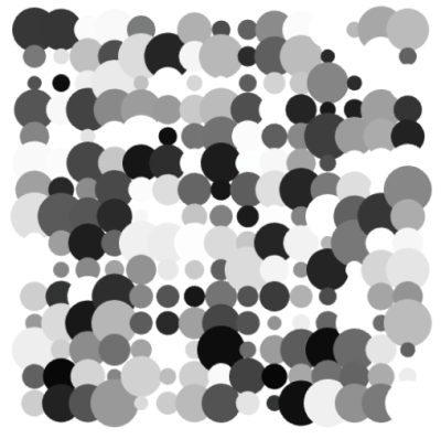
The second art assignment, as in the previous semesters, was to explore creating textures using randomness in both color and shape. As with the first assignment, I wanted students to submit one piece which involved only changing the parameters to a given function. In this case, the function created a grid of gray circles, with both the intensity of the gray and the size of the circles having some degree of randomness. I think it is important that students do some work within given constraints — it really challenges their creativity. Here is Terry’s piece along these lines.

Day112Terry

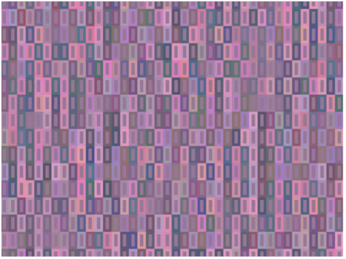
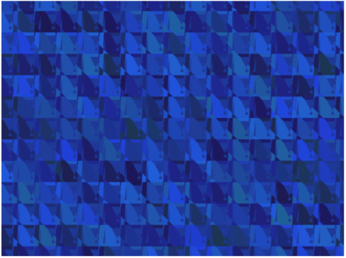
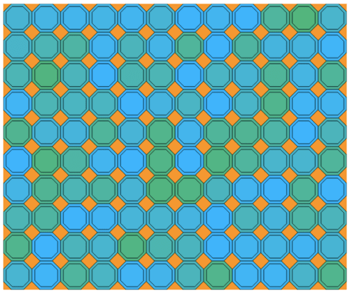
The second piece was based on a function which created a grid of squares of the same size, but random colors. Here, there were no constraints — students could modify the geometry in any way they wanted to. Several were quite creative. For example, Sepid approached this task by choosing both shape and color to create an image reminiscent of a stained glass window.

Day112Sepid

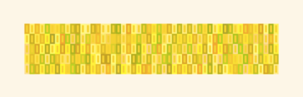
The third piece involved a color gradient (see my previous posts on Evaporation). If you look back at these posts, you’ll recall that a color gradient can be created by increasing the randomness of the colors as you move from the top of the image to the bottom using a power function: $f(y)=y$ corresponds to a linear gradient, $f(y)=y^2$ corresponds to a quadratic gradient, etc. Different effects can be created by varying the exponent.

As I was discussing this in class, one student asked what would happen if you used a negative exponent. I had never thought about this before! Jack used this idea in his piece, which he said reminds him of looking at a fire.

Day112Jack

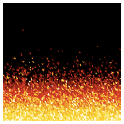
It turns out that using a negative exponent creates a gradient beginning with black on the top. Why is this? As the image proceeds lower down the screen, the algorithm subtracts values from the RGB parameters proportional to $y^n,$ where $y=0$ corresponds to the top of the image, and $y=1$ corresponds to the bottom of the image.

So if the exponent $n$ is positive, there is very little randomness subtracted. But if the exponent is negative, a lot of randomness is subtracted, since now the numbers near 0 are on the denominator. Because the RGB values only go up to 255, subtracting a large degree of randomness leaves nothing left — in other words, black. Now some of the numbers will end up being negative near the top– but putting all negative numbers in a color specification in Processing does in fact give you black.

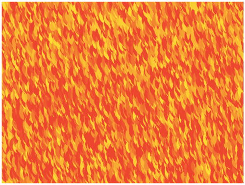
Another student also worked with yellows and reds to imitate fire in another way. Instead of making small circles, he made larger circles with quite a bit of overlap, creating a rather different effect.

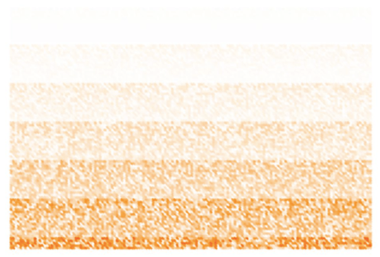
And Rosalie found in interesting say to create stripes with the algorithm. I had not seen this effect before.

Day112Rosalie

So that’s it for the first update of the Fall 2017 installment of Mathematics and Digital Art. As you can see, my students are already being quite creative. I look forward to seeing their work develop as the semester progresses!

Bay Area Mathematical Artists, I

Yesterday was the first meeting of the Bay Area Mathematical Artists at the University of San Francisco!

It all began one balmy Friday evening in Waterloo, Ontario, Canada at the Bridges 2017 conference….the Mendlers and I hosted a pot luck dinner at our AirBnB, and we realized how many of us were from the Bay area. In fact, we remarked upon the fact that nine of us were actually on the same flight from San Francisco to Toronto for the conference!

Bridges participants do really form a community. There is a spirit of sharing and mutual appreciation for each others’ work. We really do cherish those few days each year when we can all come together. The only drawback is that Bridges comes around just once a year.

So throughout the evening, between chowing down on grilled fare and sipping a glass of beer or wine, the idea of informally gathering now and then kept cropping up.

But as we all know, ideas do not automatically become reality. They have a tendency to wither if not watered and fertilized….so I decided to take up gardening.

I had the advantage of being associated with a University, so I could arrange a meeting space. Location was also somewhat convenient — some of us were to the northeast in Oakland and Berkeley, and others were to the southwest in Santa Clara and Scotts Valley. It might be nice to move around occasionally so not everyone has to drive as far all the time. But since the meetings are on Saturdays, at least traffic is not so much of a bother.

And then come the emails! Yes, lots of them…. The main decision to be made was deciding on a format. I thought informal was best — I sent out a call for speakers, and put them on the docket on a first-come, first-served basis. I wanted to take away the stress of competing for time; if there were more speakers than we had time for, we’d just start where we left off the last time.

The other reason for this is that I wanted to encourage students from my Mathematics and Digital Art class, as well as members of the newly formed Digital Art Club, to participate as well. I think it is important to let mathematical artists of all levels have a place to share ideas and get feedback on their work.

So for our inaugural meeting, we had three speakers: Chamberlain Fong, Karl Schaffer, and Dan Bach.

Chamberlain’s talk was entitled The Conformal Hyperbolic Square and Its Ilk. He discussed different ways to transform circular hyperbolic tilings (particularly those of Escher) to square images. Chamberlain did give a version of this talk at Bridges in 2016, but included more recent results as well. For more information, you can contact him at chamberlain@yahoo.com.

001title

Karl Schaffer’s talk was entitled Dance’s Center of Attention Mass. Inspired by Joseph Thie’s Rhythm and Dance Mathematics and Kasia Williams’ idea of “Center of Attention Mass,” Karl is interested in graphically showing where the center of attention is by weighting the position of each dancer on stage. He went so far as to contact Thie — now in his 80’s — and they are actively collaborating together.

Karl is also giving the lecture/demonstration Calculated Movements at the Montalvo Art Center next March. There is more information here. You can reach Karl at karl_schaffer@yahoo.com.

Finally, Dan Bach’s talk was entitled 3D Math Art and iBooks Author. Dan is keen on creating highly interactive math books which engage students of all ages. He gave a practical talk demonstrating the software he uses, including examples of converting graphics to various different formats since it is not always a simple task to take a 3D image created by one software package and import it into another. You can reach Dan at dan@dansmath.com.

DanBachSlide1

After the talks — which included ample room for Q&A — we had a brief discussion on the future of the group. I wanted to make it clear that while I am willing to keep things going in the current format, it is really up to the group to decide how to run our meetings. We opted to keep things going the same way for next month — but suggestions for the future included workshops, or perhaps themed sessions, like a series of talks on polyhedra. Participants were encouraged to think of other ways to use our time together as a topic of discussion for the next meeting. Keeping it informal means lessening the pressure of submitting talks/papers for conferences, etc.

Then dinner! Most of us were available for a meal afterwards. There were two nice options nearby — a cafe with sandwiches and salads, and an Indian restaurant with a buffet. I went with the group who preferred Indian food — and truly, a good time was had by all! We left for dinner at about 5:30, and I finally had to break things up shortly before 8:00, since some of us had a ways to drive home. We could clearly have kept talking for quite a while….

So our first meeting of the (tentatively named) Bay Area Mathematical Artists was a success! There were a total of 15 of us present, including three students from USF — a very respectable number for a first time event. We plan to meet approximately monthly, modulo the University schedule of classes and holidays.

I’ll post summaries each month of our meetings, including a brief synopsis of the talks, workshop(s), or whatever other form the meetings take. Feel free to contact the speakers for more information about the talks they gave this weekend, and don’t hesitate to spread the word to others who might be interested!

Using Processing for the First Time

While I have discussed how to code in Processing in several previous posts, I realized I have not written about getting Processing working on your own computer. Naturally I tell students how to do this in my Mathematics and Digital Art course. But now that I have started a Digital Art Club at the University of San Francisco, it’s worth having the instructions readily accessible.

The file I will discuss may be used to create an image based on the work of Josef Albers, as shown below.

0001

See Day002 of my blog, Josef Albers and Interaction of Color, for more about how color is used in creating this piece.

As you would expect, the first step is to download Processing. You can do that here. It may take a few moments, so be patient.

The default language used in Processing is Java. I won’t go into details of why I’m not a fan of Java — so I use Python mode. When you open Processing, you’ll see a blank document like this:

Day110Screen1

Note the “Java” in the upper right corner. Click on that button, and you should see a menu with the option “Add Mode…” Select this option, and then you should see a variety of choices — select the one for Python and click “Install.” This will definitely take a few minutes to download, so again, be patient.

Now you’re ready to go! Next, find some Processing code written in Python (from my website, or any other example you want to play around with). For convenience, here is the one I’ll be talking about today: Day03JosefAlbers.pyde. Note that it is an Open Office document; WordPress doesn’t let you upload a .pyde file. So just open this document, copy, and paste into the blank sketch. Be aware that indentation is important in Python, since it separates blocks of code. When I copied and pasted the code from the Open Office document, it worked just fine. But in case something goes awry, I always use four spaces for successive indents.

Now run the sketch (the button with the triangle pointing to the right). You will be asked to create a new folder; just say yes. When Processing runs, it often creates additional files (as we’ll see in a moment), and so keeping them all in one folder is helpful. You should also see the image I showed above; that is the default image created by this Processing program.

Incidentally, the button with the square in the middle stops running your sketch. Sometimes Processing runs into a glitch or crashes, so stopping and restarting your sketch is sometimes necessary. (I still haven’t figured out why it crashes at random times.)

Next, go to the folder that you just created. You should see a directory called “frames.” Inside, you should see some copies of the image.

Day110Screen2

Inside the “draw” function, there is a function call to “saveFrame,” which saves copies of the frames you make. You can call the folder whatever you want; this is convenient, since you might want to make two different images with the same program. Just change the folder name you save the images to.

A word about the syntax. The “####” means the frames will be numbered with four digits, as in 0001.png, 0002.png, etc. If you need more than 10,000 frames (likely you won’t when first starting), just add more hashtags. The “.png” is the type of file. You can use “.tif” as well. I use “.tif” for making movies, and “.png” for making animated gifs. There are other file types as well; see the documentation on saveFrame for more details.

Now let’s take a look at making your own image using this program.

Day110Screen3

If you notice, there are lines labelled “CHANGE 1” to “CHANGE 6” in the setup and draw functions. These are the only lines you need to change in order to design you own piece. You may tweak the other code later if you like. But especially for beginning programmers, I like to make the first examples very user-friendly.

So let me talk you through changing these lines. I won’t bother talking about the other code right now — that would take some time! But you don’t need to know what’s under the engine in order to create some interesting artwork….

CHANGE 1: The hashtags here, by the way, indicate a comment in your code: when your program runs, anything after a hashtag is ignored. This makes it easy to give hints and provide instructions in a program (like telling you what lines to change). I created a window 800 x 600 pixels; you can make it any size you want by changing those numbers. The “P2D” just means you’re working with a two-dimensional geometry. You can work in 3D in Processing, but we won’t discuss that today.

CHANGE 2: The “sqSide” variable indicates how big the square are, in units of pixels. The default unit in Processing is always pixels, so if you want to use another geometry (like a Cartesian coordinate system), you have to convert from one coordinate system to another. I do all this for you in the code; all you need to do is say how large each square is. And if you didn’t go back and read the Josef Albers piece, by “square,” I mean a unit like this:

Day002Square

CHANGE 3, CHANGE 4: The variables “sqRows” and “sqCols” indicate, as you would expect, how many rows and columns are in the final image. Since I have 15 rows and the squares are 30 pixels on a side, the height of the image is 450 pixels. Since my window is 600 pixels in height, this means there are margins of 75 pixels on the top and bottom. If your image is too tall (or too wide) for the screen, it will be cropped to fit the screen. Processing will not automatically resize — once you set the size of the screen, it’s fixed.

CHANGE 5: The “background” function call sets the color of the background, using the usual RGB values from 0-255.

CHANGE 6: The first three numbers are the RGB values of the central rectangles in a square unit. The next three numbers indicate how the background colors of the surrounding rectangles change. (I won’t go into that here, since I explain it in detail in the post on Josef Albers mentioned above. The only difference is that in that post, I use RGB values from 0-1, but in the Processing code here, I use values from 0-255. The underlying concept is the same.)

The last (and seventh) number is the random number seed. Why is this important? If you don’t say what the random number seed is (the code does involve choosing random numbers), every time you run the code you will get a different image — the computer just keeps generating more (and different) random numbers in a sequence. So if you find an image you really like and don’t know what the seed is, you’ll likely never be able to reproduce it again! And if you don’t quite like the texture created by using one random seed, you can try another. It doesn’t matter so much if you have many rows and columns, but if you try a more minimalist approach with fewer and larger squares, the random number seed makes a big difference.

OK, now you’re on your own…. This should be enough to get you started, and will hopefully inspire you to learn a lot more about Python and Processing!

Beguiling Games I: Nic-Nac-No

It has been some time since I’ve posted any puzzles or games. In going through some boxes of folders in my office, I came across some fun puzzles I created for a class whose focus was proofs and written solutions to problems. I’d like to share one this week.

For the assignments, I sometimes wrote stories around the puzzles. So here is one such story. The date on the assignment, if you’re interested in such things, is January 16, 2003. (I assume that you are familiar with the game Tic-Tac-Toe, as well as the fact that if both players play intelligently, the game ends in a draw.) I called the game “Nic-Nac-No.”

Betty and Clyde, after their favorite breakfast of blueberry pancakes one sunny Saturday morning, began a Tic-Tac-Toe tournament. They were reasonably bright children — taking turns going first, the initial 73 games ended in a draw.

“Just once, Clyde, couldn’t you try putting your O first on a side instead of in a corner?” prodded Betty. “That way, it wouldn’t be the same boring game every time.”

“Well, it’s my turn to go first this time,” said Clyde, putting an X in the center. “OK, now you show me how you want me to play so I can do it that way next time.”

“Oh, shut up, Clyde,” sighed Betty, putting her O in the upper left corner. And so game #74 ended in a draw.

“Hey, I’ve got an idea!” exclaimed Clyde. “Let’s make up different rules. How about this: the first one who gets three-in-a-row loses. Whaddya think, Betty?”

“That’s so random, Clyde,” said Betty, secretly excited by the suggestion.

“No, it’s not. And besides,” reasoned Clyde, “it’s got to be better than playing another game of Tic-Tac-Toe since you won’t ever try anything different.”

“OK, potato brain. Let’s try. You go first.”

“Great!” exclaimed Clyde, until he realized Betty was trying to outmaneuver him. He just realized that it you’re trying to avoid three-in-a-row, the fewer squares you own, the better.

Assuming Betty and Clyde play optimally, will the game be a win for Betty, a win for Clyde, or a draw?

I should remark that the idea of a misere game — where you turn the winning condition into a losing condition — is not original with me. But most students have not considered this type of game, so misere versions of games often make for engaging problems.

Before I discuss the solution, you might want to try it out for yourself! There are likely many strategies possible to produce the desired result; I’ll just show you the ones I thought were the most straightforward.

In my solution, Betty and Clyde use different strategies, but the end result is the same: the game must end in a draw. Let’s look at what strategies they might use.

It turns out that if Clyde starts in the center, he can use a strategy where he does not lose. It’s fairly simple: always play opposite Betty. Thus, when Betty plays a corner/side, Clyde takes the opposite corner/side.

Why can’t Clyde lose? First, it should be clear that Clyde can never make a three-in-a-row that passes through the center. Since he always plays opposite Betty, any line of three passing through the center must contain two X’s and one O (recall Clyde started with an X in the center), and so is not a three-in-a-row.

What about a three-in-a-row along a side? Since Clyde plays opposite Betty, if he ever placed an X to make three-in-a-row along a side, that would mean Betty already had three O’s in a row on the opposite side, and would have already lost! So it’s impossible for Clyde to lose this way.

Since any three-in-a-row must pass through the center or be along a side, this means that Clyde — if he plays intelligently — can never lose Nic-Nac-No.

Now let’s look a non-losing strategy for Betty. There is no guarantee she will be able to take the center square on her first move, so we’ve got to consider something different. And we can’t just rely on playing opposite Clyde, since there is no opposite move if the takes the center first. Moreover, it may be the case that Clyde uses some other strategy than the one I mentioned, so we can’t even assume that he does take the center on his first move!

To see a strategy for Betty, consider the following diagram:

Day109NicNanNo

Betty’s strategy is simple: place an O in one of the squares marked A, one marked B, one marked C, and one marked D.

Note that this is always possible. Even if Clyde does not play in the center on his first move, he can only occupy one square labelled A, B, C, or D. Then Betty places her O on the other square with the same letter. If Clyde does begin in the center, then Betty has her choice of first move.

Since it is always possible — and since Betty only has four moves — these comprise all of Betty’s moves. But note that since Betty never has an O on two of the same letter, she can never get three-in-a-row on a side. Further, since Betty’s strategy never involves a move in the center, she can never get three-in-a-row in a line going through the center square. This means that Betty can never lose!

So if the two players play their best games, then Nic-Nac-No ends up in a draw. And while these strategies do indeed work, I would welcome someone to find simpler strategies.

I’ll leave you with another version of Tic-Tac-Toe to think about. Here are the rules: if during the game either play gets three-in-a-row, then X wins. If at the end, no one has three in a row, then O wins. Does X have a winning strategy? Does O? Note that in this game, there cannot be a draw! I’ll give you the answer in my next installment of Beguiling Games….