February 2017 – Creativity in Mathematics

On Coding VII: LaTeX I

I’ll talk about LaTeX in this installment of On Coding — and my next one, too. There is so much to say, I realized I couldn’t say it all in just one blog post.

LaTeX is a markup language, like HTML, but its purpose is completely different. TeX was invented when its creator, Donald Knuth, thought the galley proofs for one of his computer science textbooks looked so awful, he thought that something should be done about it. This was in the late 70’s. TeX was initially released in 1978; in 1985, Leslie Lamport released LaTeX, which is a more user-friendly version of TeX. This Wikipedia article has a more complete history if you’re interested.

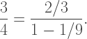
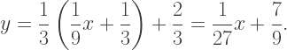
Basically, LaTeX makes math look great. Here’s a formula taken from the paper Nick and I submitted to Bridges 2017 recently.

latex1

It’s perfectly formatted, all the symbols and spacing nicely balanced. Without mentioning any names, try producing that same formula in some other well-known word-processing environment, and you’ll find out it doesn’t even come close to looking that good.

Before I go into more detail about all my favorite LaTeX features, I’d like to explain how it works. Typically, you download some TeX GUI — I use TeXworks at home. The environment looks like this:

latex2

On the left-hand side is the LaTeX markup, and on the right-hand side is a previewer which shows you how your compiled text would look as a pdf document. Just type in your text, compile, view, repeat. Much like HTML.

There are many things I like about LaTeX, and it’s hard to rank them in any particular order. Although first — and foremost — mathematical formulas look fantastic.

A close second is the fact that it’s fast. By that, I mean that because a markup language it text-based, there’s no mouse involved. I’m a very fast typist, which means I can type LaTeX markup almost as fast as I can type ordinary text. If you’ve ever hard to typeset a formula by means of drop-down menus, you know exactly what I mean.

The third feature is closely related to the second: it’s intuitive. For example, to get the trigonometric formula

$\tan\dfrac{\theta}{2}=\dfrac{\sin\theta}{1+\cos\theta},$

you would type

$$\tan\frac{\theta}{2}=\frac{\sin\theta}{1+\cos\theta}$$.

All commands in LaTeX are preceded by a backslash (“\”), so you can always distinguish them from text. And if you look at the text, you can almost figure out the formula just from reading the commands. It maps perfectly.

Most of LaTeX is that way — the commands describe what they do. For example,

$x\rightarrow y$

is created using

$$x\rightarrow y$$.

Now you might be thinking that’s a lot to type for a simple formula — surely there must be a shorter way! First, there is. You can just define your own macro by saying

\def\ra{\rightarrow}

so you could just type

$$x\ra y$$.

This might be a good thing to do if you use a right arrow all the time. But secondly, if you just use it occasionally, it’s really quite easy to remember. When you want a right arrow, you just type “\rightarrow”. If you want a longer arrow which points in both directions, like

$x\longleftrightarrow y,$

you just type

$$x\longleftrightarrow y$$.

Once you understand how the commands are named, it’s often easy to guess which one you’ll need just by thinking about it.

Next up, LaTeX makes your life a lot easier, especially when you’re working on big projects. There are a lot of ways this is done, so I’ll just mention one of my favorites — the “\label” command.

$\displaystyle\bigcup_{j\in{\mathbb Z}}{\bf R}^{2j}_{\theta}\,C_{r,\theta}^n={\bf R}^{n\,\rm{mod}\,2}_{\theta}\bigcup_{j\in{\mathbb Z}}{\bf R}^{2j}_{\theta}\,C_{1/r,\theta}^n\qquad(5)$

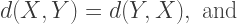
This equation (again from the Bridges paper) is typeset using the commands (broken up for reference):

\begin{equation}
\bigcup_{j\in{\mathbb Z}}{\bf R}^{2j}_{\theta}\,C_{r,\theta}^n={\bf R}^{n\,\rm{mod}\,2}_{\theta}\bigcup_{j\in{\mathbb Z}}{\bf R}^{2j}_{\theta}\,C_{1/r,\theta}^n
\label{theorem1}
\end{equation}

The equation (described by (2)) is sandwiched between a begin/end block ((1) and (4)). But the key command is the “\label” command on line (3). When you want to refer to this equation in LaTeX, you don’t use text like “equation (5)”, you say “equation (\ref{theorem1})”.

The \label command assigns the number of the equation — in this case, 5 — to the label “theorem1”. So when you use the “\ref” command (stands for “reference,” naturally), LaTeX will look for the number assigned to “theorem1”.

This might not seem like a big deal at first. But as you work on a paper, you’re always deleting equations, adding them, or moving them around. By assigning them labels, any references you make to equations in your text are automatically updated when you make changes.

And while we’re on the subject of equations — of course an extremely important topic when thinking about writing mathematics — there is also the “\nonumber” command, as well. Before you end the equation, you migh add a \nonumber tag, as in

\begin{equation}<stuff>\label{eq1}\nonumber\end{equation}.

Why would you label an equation for easy reference, and then not even put the number next to the equation? It is good mathematical style to only number equations that are referenced in the text. If you just show them once and don’t refer to them later, they don’t need a number.

But as you rewrite a proof, for example, you might find you no longer need to reference a particular equation, and so you don’t need the number any more. So rather than having to format it as not an equation (deleting the begin/end block), you just add the \nonumber tag. It’s a lot easier.

So what I do is label every equation as I write, and then when I have a final draft, I just go through and unnumber all those equations which I never end up referencing. It’s so nice.

I know I went on a bit about equations, but similar conveniences are available for figures, tables, article sections, book chapters, bibliographic entries, etc. You never have to remember a number. Ever.

And yes, there’s more…. Stay tuned for the next On Coding installment, where I’ll give you more reasons for wanting to learn LaTeX!

Mathematics and Digital Art: Update 1

I have the pleasure of teaching Mathematics and Digital Art again this semester! Since I’m largely following my outline from last semester, biweekly reports aren’t really necessary. But every month or so, I’d like to provide an update regarding changes I’ve made from the previous semester, as well as provide examples of student work.

There are no significant content changes yet — although I’ll be discussing L-systems rather than polyhedra this semester, and there will be more to say when we get to that point. But as far as the delivery is concerned, there have been some alterations.

First, I’m emphasizing the code more right from the start. You might recall that in their mid-semester comments last semester, students asked for more details about the actual coding. So I take more time in each lab explaining Python.

This change has already made an impact; I’ve noticed that students are getting more adventurous with coding earlier on. They really seem to enjoy experimenting with the geometry. The example I use for the Josef Albers assignment looks like this — just rectangles within rectangles.

sample

But Collette took the geometry quite a few steps further. In her narrative, she discussed working with figure and ground, trying to make each geometrically interesting.

I am pleased to see students playing so intently with the geometry. At first, after a detailed discussion of using two-dimensional coordinates in Python, some students just tried randomly changing numbers to see what would happen. But I encouraged them to be a little more intentional — that is, spend more time in the design stage — and they were largely successful.

The second change is that I spent an extra day on affine transformations at the beginning of our discussion, slowing down the pace a little. Last semester, I recall that I needed to go back and review ideas I thought I covered in sufficient detail. Hopefully, slowing down the pace will help.

In addition, I put together a summary of commonly used affine transformations, such as reflections:
guide

This seemed to be helpful — I used it for the linear algebra course I’m teaching as well, and students responded positively. Feel free to look at it; just go to Day 6 on the course website.

The third change involves using discussion boards more deliberately on Canvas (which is our University’s content management system). For each digital art assignment, I have students post drafts of their work, and have their peers comment on them. Since I have a small class this semester (six students), it is not a problem to have each student comment on every other student’s work.

Students really seem to enjoy this, and I participate by writing comments as well. But because everyone works at a different pace, some students lagged behind. So now I’m being more formal about using the discussion board, and making it an assignment.

For example, the next assignment involves creating three pieces, and I have assigned students to upload drafts on Canvas by the beginning of class next Friday. We’ll use Friday’s class so students can write and read comments; the assignment isn’t due until a few days later, so there will be time to incorporate new ideas into their drafts.

These changes are making a positive impact, and are making the course even more enjoyable this semester. And I am also fortunate to have Nick Mendler as my course assistant again this semester, meaning there are two of us to work with students each day. Students are really getting individual attention with their work.

Now let’s look at some more examples of student work! For the assignment to create a color texture using randomness, Lainey worked to create an image which resembled a piece of fabric.

For the Josef Albers assignment, Peyton (like Collette) also experimented a lot with the geometry of the individual elements. She chose a color palette which reminded her of a succulent, and so created geometrical objects which represented spikes on a plant.

And for the assignment based on my Evaporation piece, Karla chose a pink palette. She looked at various values for the radius and the randomness in the radius so as to create a balance between overlapping circles and white space between the circles.

karla

Stay tuned for the next update! In the next installment, I’ll let you know how the work with L-systems went. One of my favorite topics…..

A New Cantor Set?

Although we’ll do a little review, this post assumes some familiarity with the Cantor set as well as working with fractions in bases other than 10.

So what is the Cantor set?

2017-02-11cantor1

The usual geometrical definition is to begin with a line segment of length one (as shown at the top of the figure). Next, remove the middle third of that segment, so that two segments of length 1/3 are formed. Then remove the middle thirds from those segments, and continue recursively.

Even though — after this process is repeated infinitely, of course — you remove segments whose lengths sum to 1, there are still infinitely many points left! (Actually, uncountably infinitely many, although this observation is not necessary for our discussion.)

There are many ways to describe the remaining points, but one common way is to say that the Cantor set consists of all those numbers between 0 and 1 (inclusive) which, when written in base 3, may be written only with 0’s and 2’s.

Again, we’ll briefly review. We have .2₃ = 2/3_10, for example — since the places after the ternary point (no “deci”mals here) represent powers of 1/3.

So if we wanted to find 3/4 in base 3, we note that we’d need 2/3 = 0.2₃, but there would be 1/12 left over. This is smaller than 1/9, so we’re at 0.20₃ so far. Next, we need 2/27, giving 0.202₃, with 1/108 left over. And so on. The result is that 3/4 is equal to 0.202020…₃, where the “20” repeats. This can also be shown using infinite geometric series, if desired:

$\dfrac34=\dfrac{2/3}{1-1/9}.$

Surprisingly, the idea for a possibly new type of “Cantor set” came from studying binary trees! I say possibly new, since I couldn’t find any reference to such a set online, but of course that doesn’t mean someone else hasn’t come across it. And I call it a type of Cantor set since it may also be formed by taking out thirds of segments, but in a slightly different way than described above.

2017-01-02binarytree

Now I’ve talked a bit about binary trees before, so I won’t go into great detail. But here is the important idea: when you make a branch, you’re pointing in some particular direction, and then turn either left or right, but you can’t just keep going in the same direction.

So what if you looked at ternary expansions, and as you added digits, you had the option of adding 1 to the previous digit (like turning left), or subtracting 1 (like turning right), but you couldn’t use the same digit twice consecutively. So 0.21021201 would be OK (we’ll drop the 3 subscripts since we’ll be working exclusively in base 3 from now on), but 0.12002120 would not be allowed since there are consecutive 0’s.

Note that adding 1 to 2 gives 0 in base 3, and subtracting 1 from 0 gives 2. So essentially, starting with 0., you build ternary expansions with the property that each digit is different from the previous one. And, of course, the expansions must be infinite….

What do iterations of this scheme look like?

We start with a segment of length 1. Recall we begin with 0., so that means the ternary expansions may begin with 0.1 or 0.2. Expansions beginning with 0.0 are not allowed, so this precludes the first third of the segment.

Now here comes the interesting part! On the second iteration, (the third line from the top), we remove different thirds from the first two segments. Since the 0.1 may continued onto 0.10 or 0.12, but not 0.11, we remove the middle third from the 0.1 segment. Further, 0.2 may be continued as 0.20 or 0.21, but not 0.22, so we remove the last third of the 0.2 segment. The iteration process is not symmetrical.

We continue on…. Since 0.10 may be continued as 0.101 or 0.102, but not 0.100, we remove the first third of the 0.10 segment. You get the idea. Seven iterations of this procedure are shown in the figure above.

Note that since the process for creating the original Cantor set is symmetrical, this imposes a self-similarity on the set itself. The Cantor set is exactly the union of two duplicate copies of the original, scaled by a factor of 1/3.

In other words, the Cantor set may also be created using an iterated function system with the following two transformations:

$y=\dfrac13x,\qquad y=\dfrac13x+\dfrac23.$

What about the self-similarity of the new Cantor set? To help in seeing this, here’s a slightly more detailed version of the iteration scheme.

Is there any self-similarity here? Yes, but the fewest number of transformations I’ve found to describe this self-similarity is five. The curious reader is welcome to find fewer!

It isn’t hard to see the five vertical bands in this figure — the first three look the same (although the second one appears to be reflected), and the last two also look the same, although reflections of each other.

The first band is all ternary expansions in this new set beginning with 0.10. How do these relate to the whole set? Well, 1/9 of the set consists of expansions beginning with 0.001… or 0.002…, and then adding digits different from those previous. Adding 1/3 therefore gives all expansions beginning with 0.101… or 0.102…, and then adding different digits. This implies that the self-similarity describing the first vertical band is

$y=\dfrac 19x+\dfrac13.$

The second band consists of those expansions in our strings beginning with 0.12. But if x is an expansion in our set beginning with 0.10, then 1 – x must be an expansion in our set beginning with 0.12, since we may write 1 as .22222…, repeating. Therefore, the second band is represented by the transformation

$y=1-\left(\dfrac 19x+\dfrac13\right)=\dfrac23-\dfrac19x.$

We can think of the third band just as we did the first — except that this band consists of number beginning with 0.20 (rather than 0.10). So this band is represented by the transformation

$y=\dfrac 19x+\dfrac23.$

The last two bands consist of those expansions beginning with 0.21. Here, we break into the two cases 0.210 and 0.212, and use our previous work. For example, those beginning with 0.210 can be found by taking those beginning with 0.10, dividing by 3 to get expansions beginning with 0.010, and then adding 2/3 to get expansions beginning with 0.210:

$y=\dfrac13\left(\dfrac 19x+\dfrac13\right)+\dfrac23=\dfrac1{27}x+\dfrac79.$

We describe the self-similarity of the last band — those expansions beginning with 0.212 — analogously:

$y=\dfrac13\left(\dfrac23-\dfrac 19x\right)+\dfrac23=\dfrac89-\dfrac1{27}x.$

These are five transformations which describe the self-similarity of the new Cantor set. I haven’t rigorously proved yet that you can’t do it in fewer, but I think this is the case.

Of course this is just the beginning — you can use the same rule in any base. That is, begin with 0., and either add or subtract one from the previous digit. In base 4, you get nice self-similarity, but it gets more involved in higher bases. In bases higher than 3, you can also use the rule that the next digit in the expansion is different than the previous — and this gives yet another class of Cantor sets. I’ll leave you to investigate, and perhaps I’ll write again about these Cantor sets when I find out more!

What is…Taxicab Geometry?

It’s time to start exploring different geometries! Today we’ll look at taxicab geometry because algebraically, it’s the easiest one to work with. I discussed it briefly before — recall that lines and points are the same as those in the Euclidean geometry we’re used to, but the idea of distance is different. Here, the distance between two points P and Q is how far a taxi would have to drive on a rectangular grid to get from P to Q.

You can see from the figure that the distance between (-2,3) and (3,-1) is 9, since you’d have to drive nine blocks to get from one point to the other. This might seem simple enough, but the situation is quite a bit different from Euclidean geometry.

taxi1

In Euclidean geometry, the shortest distance between two points is a straight line segment. If you deviate from this segment in any way in getting from one point to the other, your path will get longer.

In taxicab geometry, there is usually no shortest path. If you look at the figure below, you can see two other paths from (-2,3) to (3,-1) which have a length of 9.

taxi2
Strange! There are a few exceptions to this rule, however — when the segment between the points is parallel to one of the axes. For example, the distance from (0,0) to (4,0) is just 4 — and there’s only one way to get there along a path of length 4. You’ve got to travel along the line segment joining (0,0) and (4,0).

Well, perhaps “strange” is the wrong word. All of this is perfectly normal in taxicab geometry….

Now let’s take a look at triangles. We define them in the usual way — choose three points, and connect them in pairs to form three sides of a triangle. Just like in Euclidean geometry.

Because we’re so familiar with them, I’ve drawn what would be — if we were in the Euclidean realm! — two 3-4-5 right triangles. You’re welcome to verify that OP’Q’ would indeed be a 3-4-5 triangle in Euclidean geometry.

OK, now let’s look at these triangles from the perspective of taxicab geometry. While we can just study these triangles by looking at the graph, it might be helpful to formally define the taxicab distance function. If two points have coordinates $P=(x_1,y_1)$ and $Q=(x_2,y_2),$ the distance between them is defined to be

$d_T(P,Q)=|x_2-x_1|+|y_2-y_1|.$

First, a word about saying that we’re defining the distance. That’s right — a different distance, like the one we’re used which comes from the Pythagorean theorem, would produce a different geometry. So how your geometry “works” depends upon how you define the distance.

Second, a word about the formula. Take a moment to convince yourself that $|x_2-x_1|$ is how far your taxicab would have to drive in an east-west direction, and $|y_2-y_1|$ is how far your taxicab would have to drive in a north-south direction. Absolute values are needed: the distances $d_T(P,Q)$ and $d_T(Q,P)$ should be positive and equal to each other.

Back to the triangles. In a taxicab world, OPQ is a 3-4-7 triangle! That might strike you as a bit unusual, since in the Euclidean world, the sum of the lengths of any two sides of a triangle is always greater than the length of the third. This is called the triangle inequality, and is usually written

$d_E(X,Z)\le d_E(X,Y)+d_E(Y,Z)$

for points X, Y, and Z, where we write $d_E$ to mean the Euclidean distance. In Euclidean geometry, the only way this inequality can actually be an equality is if Y is on the line segment whose endpoints are X and Z — and no other way. But as we’ve just seen,

$d_T(O,Q)= d_T(O,P)+d_T(P,Q),$

where P is evidently not on the segment joining O and Q. Yet another difference between taxicab and Euclidean geometries.

Oh, but it gets better…. In the figure above — at least in a Euclidean world — when you rotate two triangles, the angles and lengths remain the same. In other words, the triangles are congruent. It may seem obvious, since clearly the two triangles look the same.

What happens when we “rotate” triangle OPQ in a taxicab world? I put “rotate” in quotes since we haven’t looked at whether or not the Euclidean idea of “angle” has a companion in the taxicab world.

If you do the calculations, you’ll see that OP’Q’ is in fact a 21/5 – 5 – 28/5 triangle! Moreover, even though OQ was the longest side of triangle OPQ, OQ’ is not the longest side of triangle OP’Q’! The longest side is actually OP’.

What’s going on here? We are so used to being able to draw a triangle on a piece of paper — and certainly, if we turn our piece of paper, the lengths of the sides of the triangle don’t change! The triangle stays exactly the same — this is the notion of congruence. But when you change the distance function to $d_T,$ the geometry changes. In a very fundamental way, as you see.

Essentially, we need to give up the idea of “angle” in taxicab geometry. That might sound odd — how can you have geometry without angles? As it turns out, there are lots of ways to do this. We’ll be looking at this idea more as this thread continues.

And although there are differences, there are certainly things in common — such as the fact that there is a triangle inequality in both geometries. Is this just coincidence? Mathematically, a distance function is one which satisfies, for points X, Y, and Z:

1. $d(X,Y) \ge 0, {\rm \ with\ equality\ only\ when\ } X=Y,$

2. $d(X,Y)=d(Y,X), {\rm\ and}$

3. $d(X,Z)\le d(X,Y)+d(Y,Z).$

Now we’ve already encountered properties 2 and 3 so far, and property 1 simply says that two differents points have to be separated by some positive distance.

The concept of a distance function evolved over time — whenever it made sense to talk about distance, it seemed these properties were always in play. And in fact, the distance functions in both Euclidean and taxicab geometry have these three propertes.

So different distance functions produce different geometries. Perhaps the hardest thing about encountering new geometries is putting aside ideas from Euclidean geometry — “forgetting” all about angles, for example, while we’re in a taxicab world. Hopefully, as you learn about more and more non-Euclidean geometries, it will become easier and easier to navigate this Universe of diverse geometrical worlds….