I recently began writing some lectures for an online course — I’ll talk more about the nature of the course in next week’s post. The broad topic is geometry, of course a favorite — and the specific topic for this unit is Triangles.
You can’t talk about triangles without talking about the Pythagorean Theorem. Part of my job is also to compose problems for the lectures as well as for quizzes and exams, and to my surprise, I came up with a few interesting ones. So I thought I’d share them with you. I am always a fan of sharing mathematics as it happens!
The questions I wrote are based on the following parameterization of Pythagorean Triples: Given positive integers 

is a Pythagorean Triple. This parameterization generates all primitive Pythagorean Triples — that is, triples whose sides share no common factor. But it is not possible to get 


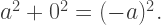
I thought of my first problem walking down the sidewalk going to lunch the other day. The simplest Pythagorean Triple, 
The simplest way to approach this is to parameterize such a triple by 


which we may rewrite as

Now this factors:

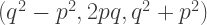
resulting in solutions 


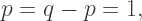
What about the solution 

which you can observe is just a multiple 

The conclusion? The only Pythagorean Triples possible whose side lengths are in arithmetic progression are multiples of the 
I really didn’t know the answer would come out so nicely — but since the algebra involved was fairly straightforward, I thought I could include this as a non-routine example of an application of the Pythagorean Theorem at the high school level.
The previous problem was part of a lecture. The next problem was written as a possible exam question for teachers; once I realized I had more than one interesting problem, I thought there would be enough for a blog post….
I was just looking for interesting patterns in Pythagorean Triples, and noticed that with the 

Of course there had to be finitely many — as the side lengths get larger, the area gets larger faster than the perimeter, as the area is essentially a quadratic function, while the perimeter is essentially a linear function. So how many others are there? Make a mental note of your guess before reading further….
We begin by parameterizing by

the factor of 
Setting the perimeter and area equal to each other results in

Cancelling out factors of 


This equation clearly has just three solutions, since one of the factors must be 

None is particularly difficult; let’s take them one at a time. When 


When 


Finally, when 


Surprised that there was just one more solution? I was! It was such a nice, straightforward solution, that I couldn’t help but include it.
There was a third problem which I liked, but the algebra was a little too intense — there was a nice geometrical solution, but it required ideas learned later on in the course. So here it is if you want a challenge: suppose you are given two right triangles, and you know that their perimeters and areas are the same. Prove that they are congruent.
I think you might enjoy solving this purely algebraically. I did like it so much, though, that I included a simpler version in one of my lectures: suppose you are given two right triangles, and you know that their hypotenuses are both of length 
To be honest, I never knew I’d find problem solving with the Pythagorean Theorem so interesting. It’s nice to know that there is always more geometry to learn! Even with something as apparently simple as the venerable Pythagorean Theorem….

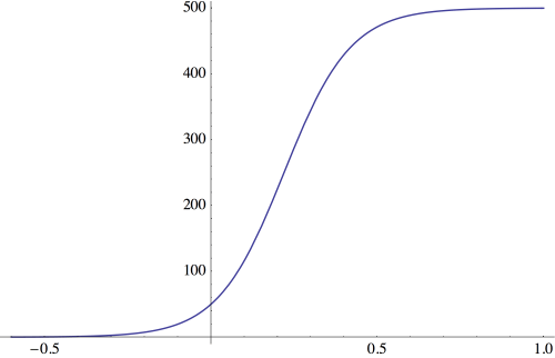
 is called the carrying capacity of the environment.
 is very small,
  and so the population growth is almost exponential. But when
  gets very close to
  then
then 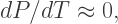 and so population growth slows down. And of course when
  growth stops — hence calling
 and
and 


 and
and  to write
 and
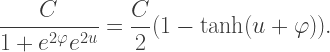
and  we need to scale by a factor of
  so that the asymptotes of the logistic curve are
 and
and 
 We can accomplish this be replacing
  with
with 


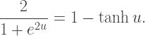
 is an odd function, becomes
 might be suggested, but how would we relate this to the exponential function?
 using the hyperbolic trigonometric substitution
  Today, we’ll look at this substitution in more depth.
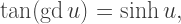
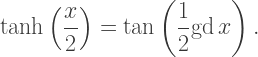
 and
and  is described by the gudermannian function, defined by
 so that this relationship is in fact invertible.
 to obtain the quadratic

 then
then  must be an increasing function of
  It is not difficult to see that we must choose “plus,” so that
  and consequently
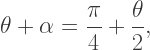
 by
by  in order to form an isosceles triangle. Thus,
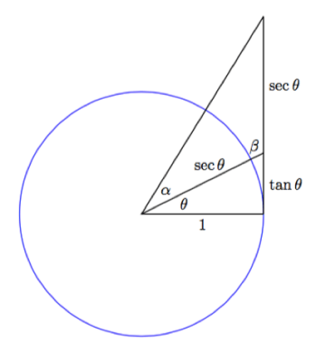
 observe that
  is supplementary to both
  and
and  so that


 giving
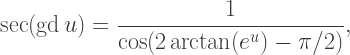


 giving
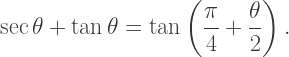
 Again using the usual circular trigonometric identities, we can show that
 and
and 
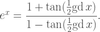
 is the inverse of the gudermannian function, then