Polyhedra Graphics, I

I decided, finally, to take the big plunge. I’ve been steadily working on my polyhedra textbook (I’ve discussed this in My Polyhedra Textbook, I and My Polyhedra Textbook, II), but ran into a bit of a snag. Since I wrote those posts, I self-published The Puzzle Cabaret, and given what I learned in the process, decided to self-publish my polyhedra book.

The snag? All my three-dimensional graphics are in color, and given that the book will approach 500 pages, would be prohibitively expensive to print in color. It would cost about $35 to print, but I want to sell it for less than that – the idea is for it not to be too expensive, so anyone with an interest in polyhedra can reasonably afford it. It would only cost about $6 to print in black and white.

The small rhombidodecahedron

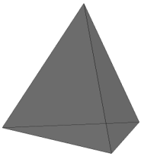
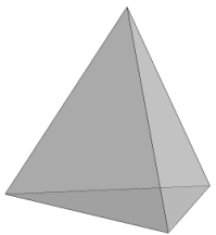
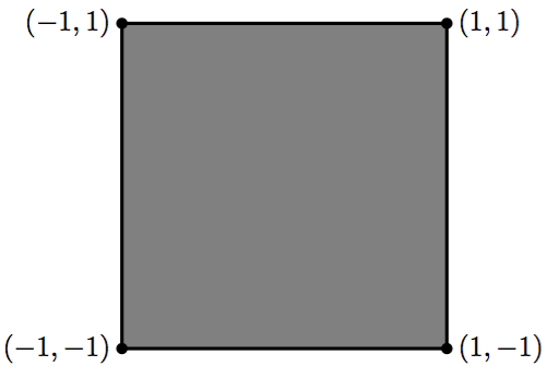
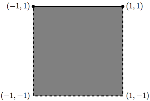
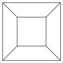
You might think, “Well, just convert to grayscale!” But what happens is that a brightly colored red tetrahedron, when converted to black and white, gives you a flat, dark gray tetrahedron — the one on the left — which is not very pleasing. And given that most polyhedra graphics on the web are similarly colored (and include some vertex/edge features which do not appeal to me), a simple conversion just won’t do. I’m looking for a tetrahedron with a little more contrast, like the one on the right.

So after a bit of work, that snag will eventually be fixed. I’ll have to redo the graphics one by one, but I have all the original code so I just need to change colors. Doable. But through conversations with Stacy (friend and design consultant), it seemed that for Part II of the book, it would be really nice to have images of all the uniform polyhedra. Really nice.

Well, I thought, that would be tons of work! Did I really think it would add that much to the book? Well, yeah, it probably would. There are programs/algorithms out there to produce polyhedra graphics, and it looked like it was time to take the plunge – dive into the inner workings of these programs and find a fairly simple way to produce the graphics. Sure, I could work them all out for myself – but data for some of the snub polyhedra require solving eighth-degree polynomials, and that’s just to get started!

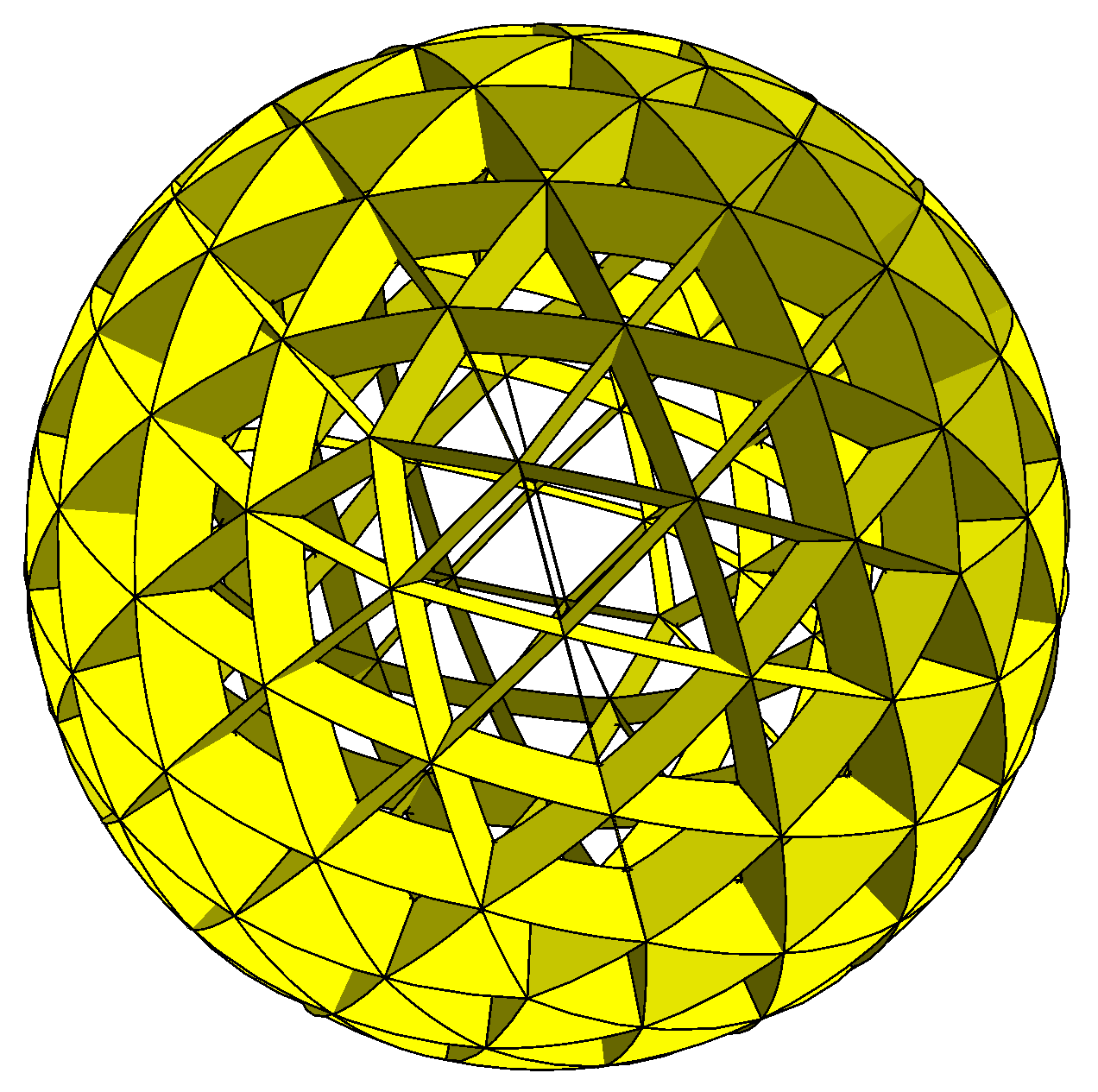
Turns out I hit the jackpot right away – and that never happens when you’re playing around with this stuff! I found this site, authored by David McCooey. For each uniform polyhedron – and its dual (when it exists) – he lists all the coordinates as well as which coordinates are vertices of which faces.

OK, that might seem like a lot of work, but I’ve worked with polyhedra graphics before. The idea is to use the symmetry of the polyhedron to help you out. So with the tetrahedron above, you just need to specify one face, and then “move it around.” In other words, use the symmetries (represented by 3-by-3 matrices) to create several different faces from one.

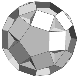
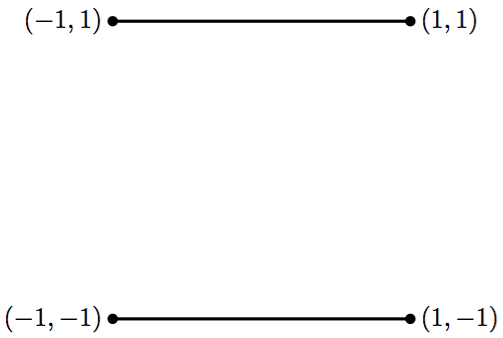
What this means is that you usually only need to specify vertices of a small number of faces, then copy them using symmetries to obtain the entire polyhedron. For example, the square and decagon below can be rotated and copied to yield the small rhombidodecahedron shown above.

So far, so good. But how do you represent the symmetries of a uniform polyhedron? Answering this question will be a major topic in this thread — I hope to walk you through a process of creating polyhedra graphics so you can try it on your own.

I’ll assume a basic familiarity with polyhedra – this thread would be impossibly long otherwise! In other words, I’ll assume that if you follow this thread, you’ve already played around with polyhedra a bit – built some, read some introductory books (like Magnus Wenninger’s Polyhedron Models, for example), and/or just stared at pictures of them, teasing out the various relationships among uniform polyhedra.

Also, I’ll need to assume some knowledge of Cartesian coordinates in three dimensions, as well as matrices and linear algebra. Anyone serious about 3D computer graphics needs this knowledge in their conceptual toolbox.

Finally, I’ll assume you’ve some programming platform you’re comfortable with which can produce three-dimensional graphics. I use Mathematica (which is not free), but I’ll discuss creating graphics from an algorithmic (rather than syntactic) point of view, so you can adapt to whatever program you’re using.

Dual of the small ditrigonal dodecicosidodecahedron

For today, I want to show you a few graphics which illustrate the basic geometry involved. If you’re very familiar with polyhedra, these ideas will not be new. But I think it’s important to include them for completeness.

The emphasis is on application, not theory. At the very least, a familiarity with abstract algebra (usually a senior-level course in an undergraduate math major) would be necessary to tackle the theory. That would be a completely different conversation, but not one for this thread.

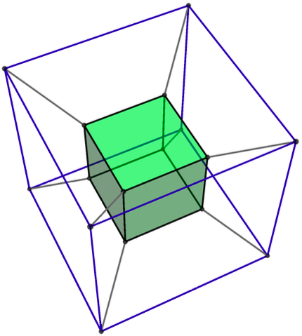
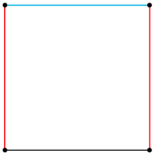
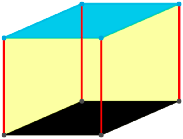
One important geometrical idea is that a tetrahedron can be inscribed in a cube, as shown below. This might not seem too amazing, but you can’t inscribe an equilateral triangle in a square in two dimensions.

Tetrahedron in a cube

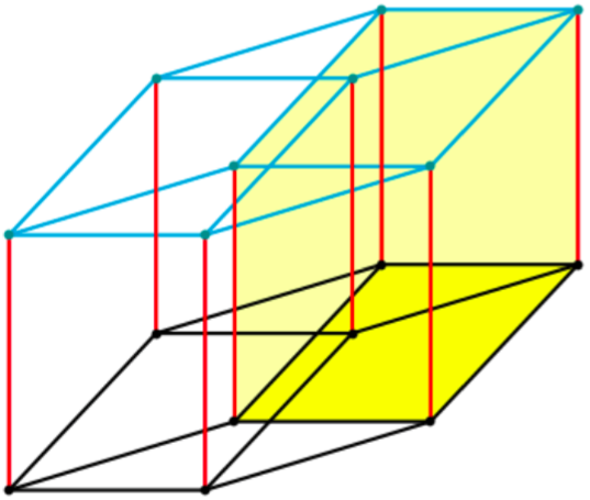
Even more importantly, two tetrahedra can be inscribed in a cube, with no vertices left over. This is truly remarkable! Of course two equilateral triangles cannot be inscribed in a square (the two-dimensional analogue), and in higher dimensions (yes, four and higher!), this does not occur either. But in three dimensions, the simple equation 2 x 4 = 8 (four vertices on a tetrahedron and eight on a cube) works its subtle magic.

Two tetrahedra inscribed in a cube

Moreover, the intersection of these two tetrahedra is an octahedron. Magic! Well, not really. It all derives from 2 x 4 = 8.

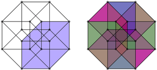
Another simple (but magic!) equation is 5 x 4 = 20. A tetrahedron has four vertices, while a dodecahedron has 20. It turns out that five tetrahedra may nicely be inscribed in a dodecahedron, as shown below. And the volume common to these five tetrahedra is an icosahedron.

Five tetrahedra in a dodecahedron

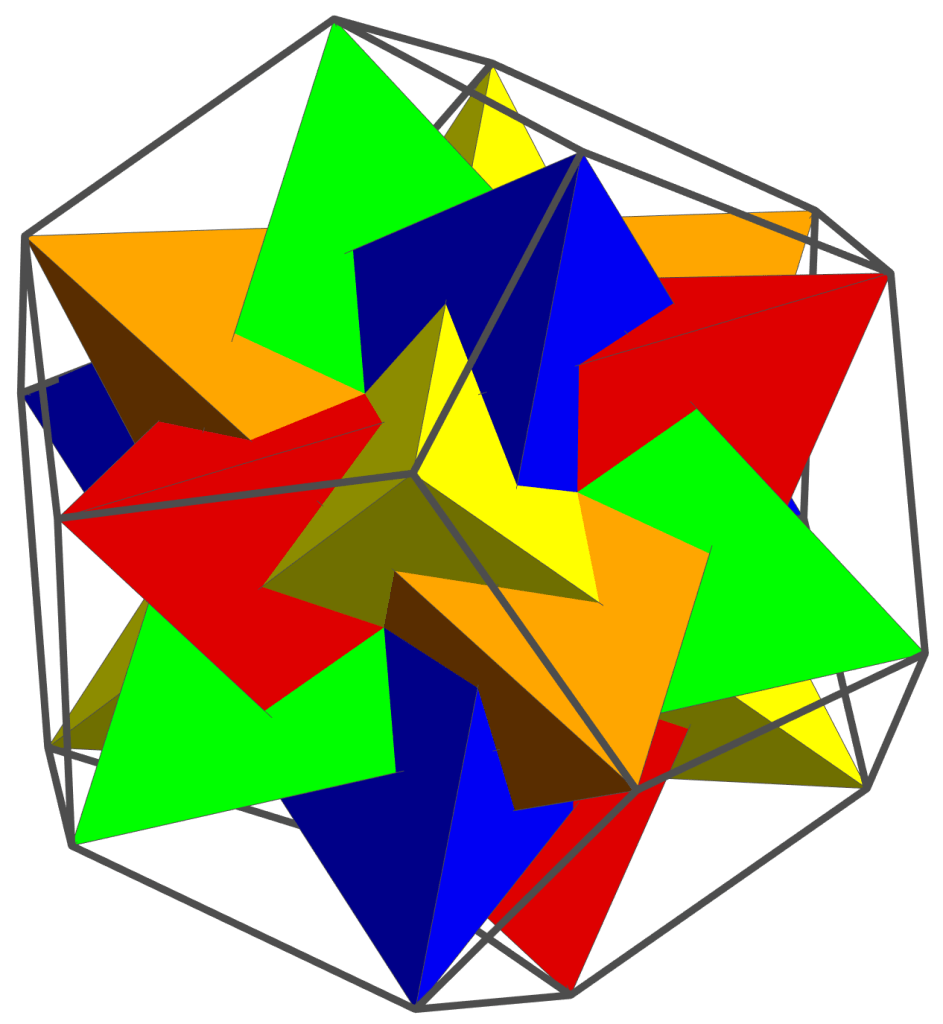
If you look carefully, you can also see that a cube (shown in light gray below) can be inscribed in the same dodecahedron. This will be a great help in finding the matrices which represent the symmetries of the dodecahedron.

Cube inscribed in a dodecahedron

This sequence of a tetrahedron inscribed in a cube in inscribed in a dodecahedron is a special feature of three-dimensional geometry. And one reason why creating polyhedra graphics in three dimensions is actually a bit easier than you might think, as you’ll see in upcoming posts….

The Puzzle Cabaret

I decided to undertake a new venture while staying home during the pandemic: write a puzzle book!

I’m not sure how the idea ultimately condensed from a gaseous nebula of random ideas, but one thought was that with so many people at home now, they needed something fun to do. Why not puzzles? With several print-on-demand platforms available, I could even self-publish!

If you’ve been following my blog from the beginning, you know I’ve written many posts about creating new and interesting puzzles. (You can search the index to easily find them.) And as a consumer of puzzle magazines for decades, I’m pretty familiar with what’s out there. Some of the current magazines include exactly the same type of puzzles they had when I was growing up.

Well, I could do better, I thought. (Although it will ultimately be up to my readers to decide that!) Since I love word, logic, and math puzzles, I’d make sure there was a nice variety. There was a particular challenge — if you look at puzzle magazines, you’ll notice that particular authors contribute the same type of puzzle to one or more different magazines. But there is just one of me.

Further, if you go to amazon.com, you might be (like I was) underwhelmed by the quality of many of the puzzle books. So I needed to create a wide variety of challenging puzzles which were not currently in circulation.

And so The Puzzle Cabaret was born! I put some sample puzzles on The Puzzle Cabaret’s website and my Twitter feed, @cre8math, so feel free to go there and check them out.

What made this such a fun project for me was that I got to use so many different tools in the toolbox I’ve outfitted over the years. Of course there is the creative task of creating new and innovative puzzles. I relied on Mathematica for some help, such as a puzzle involving words made up of three-letter words, like lithographer — LIT + HOG + RAP + HER. Rather than look through a dictionary myself, I wrote a program which searched Mathematica‘s large dictionary for 6-, 9-, and 12-letter words like this.

Or what about letters that can come before “Q” in a word? Easy to search a dictionary. I did learn a lot of new words this way — such as the only word (aside from its plural) which contains the letters “LQ” in order. Hats off to you if you know it!

So having some programming experience was helpful. My experience with mathematical art — a main thread in my blog — was helpful. I was able to do all the layout myself in LaTeX with the TikZ plugin. It’s nice because each page is essentially a sheet of graph paper — you can give exact coordinates of any page element you want so everything lines up perfectly.

I especially enjoyed creating borders around special pages — like the Table of Contents or separator pages between sections of the book. The challenge was designing something intriguing in black-and-white which would look good even if the print quality was not what you’d expect in a publisher-printed book.

Experience writing papers, books, book chapters, and teaching materials meant that I’ve become a pretty decent editor. So I could do that on my own, too. It’s tricky, though — looking at something you write over and over again. I undertook several rounds of proofreading, and kept findings things to fix each time. But at some point, you just have to stop and accept the fact that yes, there will still be a few typos in the finished book….

My design experience also meant I was able to create my own cover. It was a fun project. I went for “less is more,” and was driven by one overriding thought — my cover should shout “CLICK ME!!!” Well, I’d definitely click on it….

So having a diverse skill set was definitely helpful. But there are really so many other things which go into self-publishing a book. Learning terminology — trim size, gutter margins, embeddable fonts. Getting an ISBN. Ordering proof copies. Etc., etc. Volume 2 will be so much simpler now that I’ve finished Volume 1!

It was definitely a challenge — but one that I hope will be worth it. Because there’s the one overarching question: will anybody actually buy The Puzzle Cabaret?

I chose to sell it on amazon.com since it was the simplest marketing strategy. (Click here to see it on Amazon!) Maybe I’ll try something different for Volume 2, but my goal was to keep the monetary investment to a minimum until I knew this type of book would be popular. I really only had to pay for the ISBN, ordering proof copies, and of course paper and toner for all of the printing….

So we must let time tell! And while I was able to do a lot on my own, I must acknowledge that I have some pretty awesome friends who also have some truly exceptional skills. Stacy Speyer (see what she’s up to) was a huge help with layout as a result of her vast experience with art and graphic design. Phil Webster (see what he’s up to) play-tested many, many puzzles and gave me invaluable feedback. And Stephen Campbell (see what he’s up to) gave good advice about looking forward to future volumes.

Advice for would-be self-publishers? Patience! I’ll just give one example. Everything was going smoothly until I tried to upload my manuscript and order a proof copy to see what the final product would look like. No luck. I got some errors, and the (not-so-) helpful people at amazon.com essentially said that well, since I was using LaTeX, too bad.

Stacy came to the rescue — she’s published many books before. She just took my pdf file, uploaded it into her software, and exported it as — you guessed it — a pdf. Bingo! Of course this violates a basic mathematical principle: while 2 = 2, it is absolutely not the case that pdf = pdf. Oh, well. You get the point. With so many different variables present in the self-publishing process, something(s) will inevitably go awry. So the second piece of advice? Have smart friends!

Largest Number Found!

Late last month, Professor Warren Porterdunk of Berryville University announced that he had, in fact, found the largest number.  I was lucky enough to arrange a virtual interview with him, which is summarized here.

Of course, there is no largest number.  “That is the conventional mathematical wisdom, yes,” said Porterdunk.  “But when you include trans-transcriptional numbers — that is, numbers which cannot actually be written down — well, that’s a game-changer.”  Porterdunk calls these numbers Titans, derived from the acronym TTN, which he finds apt.

So what is the largest number?  Just a single “1” followed by infinitely many zeroes.  “That’s only one representation,” said Porterdunk.  Some real numbers have more than one representation, such as 1=0.\overline9.  The “1” followed by infinitely many zeroes — which Porterdunk calls “die Uberzahl” as an homage to Nietzsche — also has multiple presentations.  “What makes the analysis of Titans a bit tricky is that they may have uncountably infinitely many representations,” said Porterdunk.

Of course I had to ask:  What about a single “2” followed by infinitely many zeroes?  “That’s always the first question I get,” chuckled Porterdunk.  He says that the intuition which causes us to ask that question comes from the usual right-to-left algorithm for multiplying numbers.  “But the Uberzahl has no rightmost digit, so we need to throw many intuitions out the window and develop a Titan arithmetic.”

How is this done?  First, you need something called the Extendability Axiom, which postulates that (1) for a given prime number p, the limit \lim_{n\to\infty}p^n exists, and (2) if p_1<p_2, then \lim_{n\to\infty}p_1^n<\lim_{n\to\infty}p_2^n.  Porterdunk calls numbers of the form \lim_{n\to\infty}p^n, where p is prime, uberprimes.

Then, enumerate the primes, and define a Titan to be a product \prod_{n=1}^Mp_n^{k_n}, where either M=\infty or at least one of the k_n is infinite.  “The trick is to find a well-ordering on the Titans,” said Porterdunk.  “Then show that the set of Titans has a unique maximal element.  Done!”

And the trick?  Consider the uberprime P=\lim_{n\to\infty}2^n, and the Titan Q=3\cdot5\cdot7\cdot11\cdots; that is, the product of all the odd primes. Which is larger?

You might think Q is, since each odd prime is larger than 2.  On the other hand, if you look at the first two powers of 2 multiplied together, the result is larger than 3.  Then the next three together are larger than 5, the next three larger than 7, and so on.  So P must be larger.  “Consequently, you must be very, very careful when well-ordering the Titans.  Pitfalls are everywhere,” remarked Porterdunk.

A staggering 263 pages of formal proof are necessary to demonstrate that the Titans do indeed have a unique maximal element.  “Yes, the devil is in the details,” commented Porterdunk.  “One sticky point is that Titans usually have a unique factorization into finite powers of primes and uberprimes.  But quantifying what “usually” means is a very delicate task.”

Another sticky point revolves around a representation theory for Titans.  Consider the Uberzahl.  At first glance, it may seem that a “1” followed by infinitely many zeros is just the product of the uberprimes \lim_{n\to\infty}2^n and \lim_{n\to\infty}5^n.  
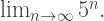
“If it helps you to sleep at night, go ahead and think that,” said Porterdunk.  “But I can assure you, there is a bit more than that to a representation theory for Titans.”  Rather an understatement, I should say!

The next steps for Porterdunk?  “I’m working on topological induction right now,” he said.  Our discussion of this was quite involved, but I’ll try to briefly summarize.  First, create a topology on the Titans such that the set of finite products of uberprimes is dense.  Then use the well-ordering to induce a Titan metric on the space.  Next, invoke the metric to define convergence in the usual way.  Then the principle of topological induction states that if Q=\lim_{n\to\infty}q_n is the limit of a sequence of Titans q_n, and if some property holds for each of the q_n, then the property also holds for Q.

“When you’ve been immersed in Titan arithmetic as I have,” said Porterdunk, “topological induction just seemed like the natural next step to take.  I think there’s a lot of potential there.”

What applications might the principle of topological induction have?  “Well, it’s very premature to make any definitive statement.  Very.  But let’s just say it might be quite interesting to several folks to know that after developing a little bit of analytic Titan theory, it may be possible to show that the Riemann hypothesis is actually equivalent to the P versus NP problem.”

Well, if that isn’t a mathematical cliffhanger, I don’t know what is!  Porterdunk said it will be a few years before he can tidy up all those details.  It definitely would be a coup for Titan arithmetic.  I’ll be sure to keep you up-to-date on this and other intriguing applications of topological induction.  Look out for the interview with Porterdunk in the New York Times next week — and don’t hesitate to visit http://www.dieuberzahl.org, where you’ll find a complete set of references and several papers to download.  I hope you’ll enjoy learning about trans-transcriptional number theory as much as I have!

Recursively Generated Spirals

A few weeks, ago I dug out a problem which had puzzled me for over three years.  I finally decided that now it was time to really dig in — and to my surprise and delight, not only did I solve the problem, but I’ve already got a draft of a paper written!  The figure below is from that paper.

Spiral

The problem is yet another variation on the recursion which produces the Koch snowflake.  I discussed the Koch snowflake in one my first posts, so visit my Day007 post on this fascinating fractal for a refresher.

So what is the variation here?  Consider the general recursive scheme

{\sf F}\ +\alpha_1\ \ {\sf F}\ +\alpha_2\ \ {\sf F}\ +\alpha_3\ \ {\sf F},

where {\sf F} represents a forward move and the \alpha_i indicate counterclockwise turns, which would be common instructions in a turtle graphics setting.

The Koch curve is generated by choosing

\alpha_1=60,\quad \alpha_2=240,\quad \alpha_3=60.

Previously I’ve studied cases where \alpha_1=\alpha_3 and the resulting image possesses central symmetry, unlike the Koch curve (see my Day008 post for examples).  But this is my first venture into exploring instances where \alpha_1\ne\alpha_3.  Things work a bit differently here….

So let’s investigate the example illustrated above in more detail.  The recursive scheme which generates this spiral is given by

\alpha_1=30,\quad \alpha_2=180,\quad \alpha_3=330.

How does this scheme draw a spiral arm?  Let’s look at the figure below.SpiralArm.png

We begin at the origin, and then draw a segment at 0^\circ, 
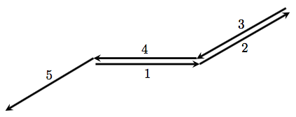
labeled “1” in the figure.  Next, we turn counterclockwise 30^\circ (since \alpha_1=30) and draw the segment labeled “2”.

The next turn is 180^\circ, so we turn completely around and begin retracing the arm in the opposite direction.  Then turn counterclockwise 330^\circ and move forward.  Note that since 330=360-30, this has the effect of taking us right back to the origin.

What next?  It is at this point that we invoke a recursive call — and so the next angle tells us what direction the next arm will be drawn in.  Of course, like before, the three angles after that will continue drawing the arm and then bring us back to the origin, awaiting the next recursive call.

This behavior can be illustrated in the following chart.

alphas.png

Here, the angles turned are listed in rows of four, one after another.  The first three angles in each row are the same, and their job is to complete the arm once a direction is chosen.  But the direction chosen is determined by the fourth column (separated by the divider), whose behavior is not periodic and highly recursive.

So where do we go from here?  The next chart we’ll look it is a chart of the directions the arms are drawn in.

Sigma4k

We read this chart in rows as follows:  the first arm is drawn at an angle of 0^\circ, directly to the right.  The second arm is drawn at an angle of 210^\circ, 
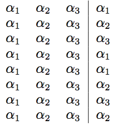
as can be seen in the figure above.

But the third arm exactly retraces the second arm drawn, since it is pointed in the direction of 210^\circ as well.  The fourth arm drawn — at an angle of 0^\circ — exactly retraces the first arm drawn.

So you can see what’s going on.  One important consequence of the recursive algorithm is that the arms keep being retraced over and over again.

When will the complete spiral be drawn?  Well, we need to see every multiple of 30^\circ in the chart above.  Of course eight rows isn’t enough.  But what is really surprising is that it takes over 1,000,000 rows before every multiple of 30 is encountered!

How would you show this?  We can’t go into all the details here.  The important observation is that if you read across the chart one row at a time, you get the same sequence of angles by reading down the first column of the chart.

But it isn’t enough to just observe this — it has to be proved.  This is where some elementary number theory comes in.  No more than what might be seen in an undergraduate number theory course, but beyond the scope of this post.

Slight step up on my soapbox — while I usually deplore the definition of mathematics as the “science of finding patterns” (as this only scratches the surface), in this case, finding patterns is critically important.  With some trial and error, you hit upon making charts in rows of four, and then putting the directions the arms are drawn in rows of four, and then stare at the numbers until you notice patterns in the charts.  The trick is knowing what to prove — once stated properly, the results almost prove themselves.

You’ll have to wait for the paper to come out for all the details.  But here is a brief summary.  Suppose you divide the circle into n parts, where n is even.  Then devise a recursive scheme using the turning angles

\alpha_1=\dfrac{360}n,\quad\alpha_2=180,\quad\alpha_3=360-\dfrac{360}n.

Now define

\sigma(k)=\dfrac13\left(4^{k-1}+2\right),\qquad k\ge1.

When n is divisible by 4, the spiral has n arms, and you need to draw exactly \sigma(n+1) 
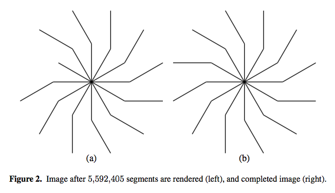
segments to render the entire spiral.  In our case, with 12 arms, it takes \sigma(13)=5,\!592,\!406 segments to render the spiral.

But when n is even but not divisible by four, the spiral only has n/2 arms, and it takes \sigma(n/2+1) segments to draw a complete image of the spiral.

Absolutely amazing, in my opinion.  I formulated these conjectures over three years ago, but got stuck.  A few weeks ago I had the house to myself for a while, and I just sat down and said to myself, “Look, you’ve already written one paper on these recursions.  You can do this.”

And within two days, I worked out the patterns.  Then the proofs, and within a week, a draft of the paper.

I am always humbled by such a seemingly innocuous problem — generating a simple spiral .  But there are so many levels to this problem, and so much interesting mathematics to be discovered.  I’ll continue exploring  recursively drawn images, and share the amazing results with you when I find them!

My Polyhedra Textbook, II

In my last post, I talked about a textbook I had written to use in a course which, among other things, introduced students to a non-Euclidean geometry — spherical geometry.  And while the primary purpose of the text was for teaching a college-level course, the actual content of the text had a different origin.

As I have mentioned previously, I got interested in polyhedra during graduate school, and was very fond of taking books about polyhedron models out of our mathematics library at Carnegie Mellon.  It was easy enough to photocopy the nets provided, or use the numerical data to construct nets on my own.

But what was missing for me, a mathematician-in-training, was a more rigorous discussion of these intriguing models.  For example, Wenninger’s Polyhedron Models contains many nets with some idea of how to construct them from a more general geometric point of view, but few details.  And his Spherical Models contains many tables of data of angular measures to three decimal places, but many derivations are missing.  Other books included metrical data such as the measures of dihedral and edge angles and circumradii, but again, often only numerically.

I should point out that this is not necessarily a criticism of these wonderful books, since each book had its own purpose.  What I found, though, was that there was really no book out there which took a more mathematically sophisticated viewpoint at an intermediate level.

So I decided that if I wanted to know more about polyhedra — that is, know the exact metrical data associated with polyhedra, not just numerical approximations — I needed to do some work on my own.

I used two approaches — coordinates and linear algebra, and spherical trigonometry.  In both cases, I wanted precise results — so typically, this meant knowing exact values for the cosines of dihedral and edges angles, for example.  When you know the cosine of an angle, you know the angle.

Why the cosine?  The sine has the disadvantage of being ambiguous, since many dihedral angles of polyhedra are obtuse — so you need more information than just the sine of the angle.  Using the tangent involved the troublesome case of \dfrac\pi2 in formulas — which occurred rarely, but was still a nuisance.  Some sources use the tangent of the half-angle, but this often involves additional calculations.

For my geometry course, I focused on spherical trigonometry — recall that I did not want linear algebra as a prerequisite for the course so that it would be accessible to a broader student demographic.  But I still wanted to keep the mathematical rigor — use spherical trigonometry to calculate exact values of the cosines of relevant angles.

To give you an idea of what’s involved, let’s calculate the dihedral angle of a dodecahedron — that is, the angle between any two pentagonal faces of a regular dodecahedron.

Fig25c

To use spherical trigonometry (see a previous post on spherical geometry for a refresher), we imagine a small sphere centered at a vertex of the dodecahedron — it will carve out a spherical triangle, as shown below.

sphdodecahedron

Here, a is a vertex of the dodecahedron, and points b, c, and d are the points where the small sphere intersects the edges of the dodecahedron meeting at a.  This creates a spherical triangle whose sides all have measure 108°, since the interior angles of a regular pentagon all have measure 108°.

The angles between the sides of the spherical triangle with vertices a, b, and c are the dihedral angles of the dodecahedron, whose measure we call D.  We may apply the law of cosines for spherical triangles in order to find (see the relevant Wikipedia page; in the textbook, spherical trigonometric formulas are discussed in detail):

\cos108^\circ=\cos108^\circ\cos108^\circ+\sin108^\circ\sin108^\circ\cos D.

To find \cos D, we need to know the following (also explained in the text):

\cos108^\circ=\dfrac12(1-\tau),\quad\sin108^\circ=\dfrac12\sqrt{\tau+2},

where \tau 
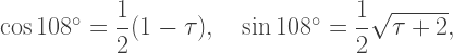
is the golden ratio.  (I use \tau for the golden ratio as this is the notation Coxeter used in his well-known Regular Polytopes, which inspired generations of polyhedral enthusiasts.)

Solving yields

\cos D=-\dfrac1{\sqrt5},

so that D is approximately 116.6°.

Now this is not the only way to find D; it is possible to find Cartesian coordinates for the vertices of the dodecahedron and use some linear algebra, for example.  But using spherical trigonometry is straightforward and elegant — and is surprisingly versatile.

When I teach my polyhedra course, we use spherical trigonometry to find edge and dihedral angles of all the Platonic and Archimedean solids.  Further, we use spherical trigonometry to design geodesic models, like the 4-frequency icosahedron shown here.

Fig47b.png

So the emphasis is on applying spherical trigonometry to the construction of physical models.  In a typical two-lecture-per-week course, one lecture is always a hands-on laboratory, where we build a polyhedron or geodesic model we studied previously.  We never build a model without knowing precisely how it is designed — we first understand the mathematics of the model, and then we build it.  Included in the text is a week-by-week outline of how I’ve used the text in the classroom.

Now the classroom textbook is just Part I of the book.  Part II is a bit more technical, and intended for the true polyhedral enthusiast.  It turns out that spherical trigonometry is a powerful tool for studying polyhedra.  In fact, the dihedral angles of all the uniform polyhedra may be calculated using spherical trigonometry — even the most complex snub polyhedra.  However, it is sometimes necessary to solve sixth-degree polynomials in order to do so!

I thought to add Part II to the volume as I had already done all the calculations some years ago.  And, to my knowledge, the calculation of the dihedral angles of all the uniform polyhedra using spherical trigonometry has not been published before.  So I hope to contribute something to the literature of classical polyhedral geometry by publishing this book, in a way that someone with a modest mathematical background can understand.

As I continue with the book project, I’ll post updates as I discover interesting geometrical tidbits along the way!

My Polyhedra Textbook, I

Now that I’ve moved on to semi-retirement, there is time to take on a 25-year-old project:  my textbook on polyhedra!

I became interested in polyhedra during graduate school, when I was fascinated by the trio of books by Magnus Wenninger:  Polyhedron Models, Dual Models, and Spherical Models.  I don’t know how many times I checked out Polyhedron Models from the mathematics library at Carnegie Mellon University, but I have clear memories of flipping pages back and forth over and over again, trying to understand the various and subtle relationships among the 100+ models shown in the book.

Of course this prompted me to build my own models — but at a time when there weren’t nets available online.  So I designed my own nets using Postscript.  Since I loved coding, this was no problem at all.  I essentially wrote my own turtle graphics package in Postscript, and used this to create any net I wanted.

Having moved around several times in recent years, I have very few models that I’ve built.  And like many model builders, I’ve given most of them away, anyway.  But here are a few I made for my friend Sandy (whom I’m visiting as I write this post).


Eventually I finished graduate school and went on to my first university teaching position, where I stayed for fourteen years.  I was at a small, liberal arts school, where many of the mathematics majors were destined to be middle school or high school mathematics teachers.  Moreover, I was to replace a retiring faculty member who had taught a course entitled, “Higher Geometry.”

I eagerly agreed to take on this mantle, but was interested in shifting the focus.  In particular, I wanted to make the course about polyhedra rather than the usual content of a Higher Geometry course, which often included a lengthy discussion of hyperbolic geometry.

Allow me a moment to step on my pedagogical soapbox here.  Yes, I understand the importance of introducing students to a non-Euclidean geometry.  But as many of my students were prospective teachers, I knew there was really no way they would be able to introduce hyperbolic geometry to their students.

But spherical geometry is also an example of a non-Euclidean geometry, and further, you can actually build physical models of non-Euclidean objects by building geodesic models.  So while you can’t really see that a triangle in hyperbolic geometry has an angle sum less than 180°, you can actually see that a spherical triangle has an angle sum greater than 180°.

You can also look at axiomatics in spherical geometry, with the added bonus that you expose students to the important concept of duality.  Finally, you can ramp up the mathematical content of such a study by introducing students to spherical trigonometry.  I should remark that, very likely, fewer than 1 in 10 (or perhaps even 1 in 100) mathematicians can rattle off the cosine law for spherical triangles — so exposing students to spherical trigonometry is significant.  It’s practical as well — think of flight paths — but I never went into this application as there just wasn’t enough time.

Stepping off my soapbox now…suffice it to say that I was given free reign to retool the Higher Geometry course.

I decided to have the course be centered on spherical trigonometry.  Why?  First, the course needed some substantial mathematical content; spherical trigonometry can be quite challenging, especially some of the more involved derivations.  This also allowed for a fairly detailed study of polyhedra, as the edge and dihedral angles of all the uniform polyhedra can be found using spherical trigonometry.

Now it is possible to find edge and dihedral angles of polyhedra in other ways, but these usually involve linear algebra applied to Cartesian coordinates in three dimensions.  And in the typical undergraduate curriculum, linear algebra follows the calculus sequence.

So if I wanted the course to be accessible to other students — such as those needing a mathematics elective but were too advanced for, say, college algebra — I couldn’t have linear algebra as a prerequisite.

And so a new “Higher Geometry” was born.  I did eventually rename the course to “Polyhedra and Geodesic Structures,” as it was more apt — one main application of spherical trigonometry I introduced was building spherical models, like those described extensively in Wenninger’s Spherical Models.  It was a highly successful course, which I taught off and on at various institutions for about twenty years.  I also conducted any number of workshops for both teachers and students of all ages over the same time span.

Essentially, students and teachers of all ages just loved the hands-on aspect of building polyhedra and spherical models.  They often commented on how building their own models made mathematics “real.”  There was always the added bonus that they got to take their work home with them!

Yes, model building is a fun activity.  But I always made sure to balance content with the hands-on laboratory experience.  We never built any models without understanding some aspect of the geometry underlying the models.

Naturally, that geometry varied with the students involved.  For middle school students, working with spherical trigonometry was far too advanced.  But we could always see how Euler’s formula applies to convex polyhedra.

In my university-level course, we actually proved Euler’s formula using spherical geometry with the method attribute to Legendre; despite others’ claims to the contrary, it is in fact the most elegant proof of Euler’s formula….

And this is just the first part of the book!  In my next post, I’ll say a little more about the genesis of the first part, and then go on to describe the second part of the book.  Expect a long thread about polyhedra and three-dimensional geometry in the upcoming months….

The Fourth Dimension, IV

In the past few weeks, we looked at the hypercube in four-dimensional space.  We approached this intriguing geometrical object using thinking by analogy; that is, we looked at one-, two-, and three-dimensional hypercubes (segments, squares, and cubes), and imagined potential properties — such as the number of vertices, edges, faces, and cells — of a four-dimensional analogue.

Moreover, we made these counts in two different (although related) ways, and obtained the same results.  We ended last week’s discussion with the following question:  yes, we obtained these counts in two different ways, but exactly what were we counting?  In other words, what was this hypercube we were analyzing?  Did we make the extension into four dimensions in a mathematically sound way?

We won’t be able to go into all the details in this post, but we’ll outline the main ideas which suggest that our reasoning so far in the series to this point could be made rigorous.

So what we need to do is actually say just what a hypercube in four dimensions actually is.  There are different ways to make this precise, but perhaps the easiest way is to use Cartesian coordinates.  Most readers are likely fairly familiar with representing a point in the plane by the Cartesian coordinates (x,y), and many have encountered (x,y,z) as a representation of a point in three-dimensional space.

What about four-dimensional space?  It is natural to just “add” another coordinate, and represent a point in four-dimensional space by (x,y,z,w) (yes, the “w” comes last, so the other coordinates continue to make sense in the usual way).

You might ask, how can we just add another coordinate?  In other words, how can we just add a dimension?  To do this rigorously, we would need to study some linear algebra — in particular, the geometry of n-dimensional real space, usually denoted by the symbol “{\mathbb R}^n.”  In the general case, we have lists of n real numbers representing points in an n-dimensional real space.

So let’s take this point for granted, and do a little more thinking by analogy.  Or perhaps it might be better to say “defining” by analogy.  For example, we might define a square, together with its interior, as

\{(x,y)\,:\,|x|\le1,|y|\le1\}.

Now this certainly seems a bit more complicated than how a square is typically defined in elementary geometry.  But this set of points is easy to sketch in the plane.  Moreover, given this algebraic description of the square, it is easy to enumerate the vertices:  (1,1), (-1,1), (-1,-1), and (1,-1).

Day173Square.png

Alternatively, the set containing these four vertices is given by

\{(x,y)\,:\,|x|=1,|y|=1\}.

Moreover, we can algebraically describe the top edge of square:

\{(x,1)\,:\,|x|\le1\}.

But do you see the catch?  Suppose we are given an algebraic description of a set of points in the plane, such as the square above.  How do we algebraically define its vertices?  edges?

Ask yourself the following question:  can you find a point in the set described above — the square — which has the property that there exists a line which intersects the square in only that point?  The answer is yes:  but such a point must be a vertex of the square.  So we might use this property to define the vertices of a set.

But we must be careful.  With this definition, every point on this pair of line segments would then be a vertex!

Day173Square2

This is certainly not what we want.   To see how to address this issue, we might introduce another concept:  convexity.  You might remember this idea coming up in my post about polygons, but here is a brief refresher.  A convex set has the property that the segment joining any two points of the set lies entirely within the set.

Day106Convexity

Using polygons as examples, the two polygons on the left would be convex, but the two on the right would not be convex.

This idea generalizes into any number of dimensions; but we’ll look a little more at two dimensions right now.  Looking back at the picture of the square, and the picture of the two line segments, we observe that the square is a convex set, while the pair of segments is not.

So we might be tempted to say that if a set is convex, then any point which is the intersection of that set and some line is a vertex of the set.  This works for the square, but…consider the circle shown below.

Day173circle

Are there points which are the intersection of this convex set and a line?  Yes there are — any point on the boundary of the circle, since a tangent line to a circle always intersects the circle in a single point.

So does a circle have infinitely many vertices?  In this case, we would actually call points on the circle extreme points of the convex set.  So a vertex would be just one example of an extreme point of a convex set.

Now what about the convex set here?

Day173Square3

The dashed lines indicate that part of the boundary is missing.  This set has just two extreme points, not four.  The problem here is that this set is not closed in a topological sense.  I won’t say more about topology here — it’s quite a huge topic! — but you can see that the number of vertices on a “square” depends critically upon whether the boundary is included.

I hope you can see that there are several issues involved in gleaning geometric properties from a purely algebraic description.  But the point is this:  we may define a hypercube as the set

\{(x,y,z,w)\,:\,|x|\le1,|y|\le1,|z|\le1,|w|\le1\}.

This is a completely unambiguous definition, but the difficulty lies in describing geometrical properties of a set using only rigorous mathematical definitions and not relying on what it looks like.

So this is why, mathematically, we can say just what a four-dimensional hypercube really is.  It takes a bit of work to tease out all the properties of a hypercube, but it can be done.

And no, this isn’t the only way to define a hypercube either….concepts such as convex hull or Cartesian product may be used to give other descriptions as well.  Feel free to look these ideas up if you’re interested in learning more about them….


The Fourth Dimension, III

Last week we counted vertices, edges, faces, and cells on a hypercube.  Mainly, we thought by analogy — but how could we be sure our intuition was correct?  Today, we look at another say to make these same counts, and obtain the same results.  This suggests that maybe we were right all along….

So we begin by looking at the square and cube in a different way, and thinking (again) by analogy from there.

Let’s start with the number of edges on a square this time. We’ll start with one dimension less than the object we’re examining — later we’ll use the squares on a cube, and the cubes on a hypercube.  Now to count vertices, we note that each edge has two vertices — for 4 x 2 = 8 vertices.  But when we join the edges at vertices, two vertices merge, so we’ve overcounted by a factor of 2.  Thus, there are 8 / 2 = 4 vertices on a square (as we know).

What happens when we look at the cube in the same way?  Let’s start with the six squares.  To count edges, we see that each square on the cube has 4 edges, for a total of 6 x 4 = 24 edges.  But as with the vertices on the square, when we join two squares at their edges, two edges merge, so we’ve overcounted by a factor of 2.  This means there are 24 / 2 = 12 edges on the cube.

For vertices, we note that three squares meet at each vertex.  So there are  6 x 4 = 24 vertices on the 6 squares — but when we join the squares together, three vertices merge to one.  This means we’ve overcounted by a factor of 3, so there are 24 / 3 = 8 vertices on a cube.

Now begin with the eight cubes on a hypercube.  We note that the “8” comes from the sequence 2, 4, 6, 8,… for 2 vertices on a segment, 4 edges on a square, 6 squares on a cube, etc.  On the square, we saw that 2 vertices merged.  On the cube, we observed that 2 edges merged, then 3 vertices.  By analogy, on the hypercube, we should have 2 squares merging, 3 edges, and 4 vertices.  This pattern continues into higher dimensions as well.

Let’s use this analogy to check that we’ve counted correctly.  First, we count squares.  With 8 cubes, we have 8 x 6 = 48 squares.  But since the cubes meet square-to-square, we’ve overcounted by a factor of 2, so that there are just 48 / 2 = 24 squares on a hypercube.

Now on to the edges.  Since 8 cubes contribute 12 edges each, there are 96 edges in total.  But three cubes meet at each edge, so we’ve overcounted by a factor of 3.  This implies that there are in fact 96 / 3 = 32 edges on a hypercube.

Finally, we count the vertices.  With 8 vertices on each of 8 cubes, we have 64 vertices all together.  But four cubes meet at each vertex, so we have in fact overcounted by a factor of 4.  This results in just 64 / 4 = 16 vertices on a hypercube.

So we counted correctly!  Well, almost….  You might have noticed that we haven’t exactly defined what a hypercube is in a rigorous mathematical way.  Until we do, the best we can say is that we’ve counted something, although we don’t know precisely what they something is at the moment.  That will be a subject for a later post.

As you might expect, there are other ways to represent a hypercube besides the figure shown in last week’s post.  We chose that particular representation because of the way we were thinking by analogy.

We’ll look at two additional ways.  The first is analogous to looking at a cube face on, as shown below.

Day172Hypercube1

Of course the inner and outer squares are the same size on a cube — but we can’t help distorting faces of the cube when we make a two-dimensional sketch.  Four of the squares are distorted into trapezoids here.

Here is the analogous representation of the hypercube.

Day172Hypercube2

In this figure, the inner cube (in green with black edges) is in fact the same size as the outer cube (with blue edges); these cubes are directly opposite each other on the hypercube.  This is directly analogous to the inner and outer squares we saw in the earlier figure.

Further, note how the other six cubes are distorted into frustums of square pyramids — you can easily see the trapezoidal faces, which we also saw in the earlier figure.  If you look carefully, you can count the 16 vertices and 32 edges.  The 24 squares are a bit trickier — but begin with the 12 squares on the inner and outer cubes.  Each of the other 12 squares contains exactly one black edge and exactly one blue edge — they are going “out” from the black edges to the blue edges.  The perspective is different, but all the squares are there.

And of course there are the eight cubes — the inner cube, the outer cube, and the six frustums of square pyramids.  All the elements of the hypercube are indeed present, but again, in a different perspective.

I did save the best for last — my favorite representation of a hypercube, shown below.

Day172Hypercube3.png

I just love the symmetry of this image — the octagram inside the octagon.  If you look at the left image, you’ll see one of the eight cubes highlighted in blue.  When each of the eight cubes is transparently colored in the right image, you’ll see an interesting overlap of colors.

Now let’s count the vertices, edges, faces, and cells in this figure.  The 16 vertices are readily apparent in the inner octagram and the outer octagon.  The 32 edges can be seen by counting eight edges from both the octagram and octagon, and two additional edges connecting each vertex of the octagon to two vertices of the octagram.

The squares are a bit trickier here as well — but eight are easily visible as undistorted squares sharing one edge of the octagon.  But if you look carefully, you’ll also see 16 additional squares as rhombi in the figure.  Eight of these rhombi each share two edges with the octagon, and the eight others each share two edges with the octagram.  It might take staring for a minute, but they are all there.

And finally, there are the eight cubes. As seen in the left image, three consecutive edges of the octagon are enough to determine one of the cubes. Since we can take three consecutive edges of an octagon in exactly eight ways, we have found the eight cells on the hypercube.

So again, all the elements of a hypercube are present — it just takes looking from the right perspective to see them all.

Still remaining is to obtain the same counts by considering a rigorous definition of a hypercube.  That for a later post….

The Fourth Dimension, II

Last week, I introduced the idea of a fourth spatial dimension.  The typical question students ask is simply, “Where is it?”  These doesn’t seem to anywhere it can go — and in fact, since we live (insofar as we know it) in a three-dimensional world, there really isn’t anywhere it can go.

So the fourth spatial dimension must be, for us, an abstraction.  To think about it, we must somehow relate it to things we already know — in particular, geometry in dimensions zero, one, two, and three.  Therefore, to think about the tesseract — the four-dimensional analogue of the cube — we must somehow think by analogy.

In particular, we can think about how we go from a point (zero dimensions) to a line segment (one dimension), and then from a line segment to a square, a square to a cube, and then make the analogous leap from a three-dimensional cube to a four-dimensional tesseract, or hypercube.  We’ll look one way to do this in today’s post, and next week, we’ll see a different way.  It’s a good idea to look at this “new” fourth dimensional from different perspectives to make sure our thinking by analogy is accurate.

To create a line segment from a point, we think of it moving one unit (we need to be specific) along a “new” first dimension to create another point — these two points are vertices of the line segment, and one edge is created.

Now move this segment one unit along a second dimension which is perpendicular to the line segment, as shown below.

Day171a.png

Now let’s count.  We have two vertices and one edge for each of the two segments (the one at the bottom in black, and the one at the top in blue), and each vertex creates another line segment (shown in red above) as it moves from the bottom segment to the top segment.  This gives a total of four vertices and four edges on a square — as expected.

Thinking by analogy, we now imagine a square moving up along a perpendicular dimension, as shown below.

Day171b

Counting vertices, edges, and faces, we have 8 vertices, 8 edges, and 2 faces from the bottom and top squares, shown in black and blue, respectively.  Now each vertex of the bottom square creates an edge as it moves up (creating 4 more edges, shown in red), and each edge of the bottom square creates a new face (creating 4 new faces, shown in pale yellow).  This gives a total of 8 vertices, 12 edges, and 6 faces.  Notice the strategy: count the bottom and top figures, and then notice what is created by vertices and edges as they move along a perpendicular dimension.

Now it’s time to extend this strategy into the fourth dimension.  To do so, we need to imagine a cube moving out along a fourth spatial dimension — and of course, it is difficult to imagine because we are so used to our three-dimensional world.

Day171c.png

Look at the above figure.  Let’s think of the cube outlined in black as the base cube.  Move this cube out along a fourth spatial dimension — so that each vertex creates an edge (shown in red) as it moves to the top cube (shown in blue).

Before we start counting, we need to introduce a little terminology.  The four-dimensional analogue of a polyhedron is called a polytope, and in addition to vertices, edges, and faces, we have three-dimensional cells on a polytope.

Now let’s count the vertices, edges, faces, and cells on a hypercube in just the same way as in the previous two examples. For vertices, we have 16 total — 8 from the base cube, and 8 from the top cube.  For the edges, we have 12 each for the base and top cubes, and each vertex of the base cube creates a new edge (shown in red).  This gives a total of 12 + 12 + 8 = 32 edges on the hypercube.

What about faces?  Well, we have 6 faces each for the base and top cubes, and each edge of the base cube creates another square face (as it did when we created the cube).  This gives us 6 + 6 + 12 = 24 faces.  Finally, to count the cells, we have the base and top cubes, and each square face of the base cube moves out to create another cube (such as the one shown in yellow, with the square from the base cube shown in darker yellow).  This gives 2 + 6 = 8 cells (cubes) on the hypercube.

How can we be sure this is correct?  Next week, we’ll look at a different (though certainly related) way to count the number of vertices, edges, face, and cells on a hypercube.  We will see that we do in fact obtain the same counts.

As a final remark, we briefly look at Euler’s Formula in four dimensions.  Recall that V-E+F=2, where V, E, and F represent the numbers of vertices, edges, and faces on a convex polyhedron.  Now if C represents the number of cells on a polytope, the four-dimensional analogue of Euler’s Formula is

V-E+F-C=0.

In our case, we have the true statement

16-32+24-8=0.

We won’t go into more depth here, as that would take us quite a bit further afield.  But if you’re interested to know more, you can always look up Euler’s Formula in higher dimensions, and extensions which have to do with the topology of geometrical objects, which is fairly straightforward when the objects are convex.  When they’re nonconvex, the situation is decidedly more difficult.

Stay tuned for next week’s post, where we look at yet another way to count the numbers of vertices, edges, faces, and cells on our friendly tesseract!

The Fourth Dimension, I

I have found that the topics of infinity and the fourth dimension really do always pique students’ interest.  When I had a few moments left at the end of a class period, I could sometimes casually remark about one of these topics, and I immediately had the attention of the entire classroom.

One of my projects has been writing an introductory book on polyhedra, and I’m in the middle of a proposal to have the book published.  A draft chapter was on the fourth spatial dimension, so I thought I’d share it here.  As much as I love the topic, I rather surprised myself by looking at my blog index and finding I’d never talked about it before….

What follows is the draft chapter, slightly edited as a stand-alone series.  Enjoy!

“What is the fourth dimension?

No, it’s not time.

Well, maybe it is if you’re studying physics.  Even then, we have certain intuitive ideas about how time works.

For example, if I imagine that it’s 9:17 a.m. in San Francisco, then I know what time it is in any other city in the world.  In New York City, it must be 12:17 p.m., since I add three hours to convert to Eastern Standard Time.

This assumption is just fine for getting along in daily life — and as far as most people are concerned, this way of thinking about time is right.  But in fact, it works only because in our daily lives, we move around fairly slowly — at least compared to the speed of light.

To understand what happens when particles do move close to the speed of light, you need to study special relativity — and here, our ordinary intuitions about time are no longer valid.

But we’re interested in a fourth spatial dimension.  How is this possible?  Where is it?  We are so used to living in a three-dimensional world, the idea of a fourth spatial dimension seems rather fantastic.

In 1884, Edwin Abbott’s delightful novella Flatland was published (Abbott, Edwin A. Flatland: A Romance in Many Dimensions. New York: Dover Thrift Edition. 1992).  The protagonist was none other than A Square, an inquisitive four-sided being living in a purely two-dimensional world called Flatland.

He was chosen as the Flatlander to receive a visit from a Sphere on the eve of the Third Millenium.  This was an unnerving visit for A Square, since the Sphere kept suggesting he consider the direction upward, but there was no upward for A Square.  There was North, South, East, and West, but A Square just couldn’t fathom this direction, “upward.”

Finally, the Sphere lifted A Square out of his two-dimensional world to show him the glory of Space.  Quite a revelation!

We are in the same predicament as A Square when it comes to contemplating a fourth spatial dimension.  Yes, we can look forward, backward, to our left and right, up and down, but nowhere else.  It doesn’t seem that there is enough room for a fourth dimension.  Where would it be?

In a typical high school geometry class, you would likely have been introduced to points, lines, and planes — and perhaps were told that points are 0-dimensional, lines are 1-dimensional, planes are 2-dimensional, and that all objects of these types live in a 3-dimensional space.  But while there were infinitely many points, lines, and planes, there was only one 3-dimensional space.

And while we do not encounter a fourth spatial dimension on a daily basis, we don’t actually encounter points, lines, or planes, either.  Can we actually see a point if it has no length?  How could we possibly see a line if it has no width?  It would be invisible.  These geometrical ideas are in fact mathematical abstractions — and once we enter the world of mathematical abstraction, our universe becomes almost unimaginably vast. A. R. Forsyth wrote almost one hundred years ago (A. R. Forsyth, Geometry of Four Dimensions, Cambridge University Press, New York, 1930, p. vii.):

Mathematically, there is no impassable bar against adventure into spaces of more than three dimensions of experience.

To get a handle on how to imagine the fourth dimension, we’ll look at one of the most popular and well-know denizens of that rarefied world — the hypercube, also known as a tesseract.”

What follows is an extended example of “thinking by analogy,” which would make this post much longer than I usually allow myself.  So that’s where we’ll start next week!