Still more on: What is…Inversive Geometry?

Now for the final post on inversive geometry!  I’ve been generating some fascinating images, and I’d like to share a bit about how I make them.

2017-07-19Inversion3v2.png

In order to create such images in Mathematica, you need to go beyond the geometrical definition of inversion and use coordinate geometry.  Let’s take a moment to see how to do this.

Recall that P′, the inverse point of P, is that point on a ray drawn from the origin through P such that

[OP]\cdot[OP']=1,

where [AB] denotes the distance from A to B.  Feel free to reread the previous two posts on inversive geometry for a refresher (here are links to the first post and the second post).

Now suppose that the point P has Cartesian coordinates (x,y).  Points on a ray drawn from the origin through P will then have coordinates (kx, ky), where k>0.  Thus, we just need to find the right k so that the point P'=(kx,ky) satisfies the definition of an inverse point.

This is just a matter of a little algebra; the result is

P'=\left(\dfrac{x}{x^2+y^2},\dfrac{y}{x^2+y^2}\right).

What this means is that if you have an equation of a curve in terms of x and y, if you substitute x/(x^2+y^2) everywhere you see x, and substitute y/(x^2+y^2) everywhere you see y, you’ll get an equation for the inverse curve.

Let’s illustrate with a simple example — in general, the computer will be doing all the work, so we won’t need to actually do the algebra in practice.  We’ll look at the line x=1.  From our previous work, we know that the inverse curve must be a circle going through the origin.

Making the substitution just discussed, we get the equation

\dfrac x{x^2+y^2}=1,

which may be written (after completing the square) in the form

\left(x-\dfrac12\right)^2+y^2=\dfrac14.

It is not hard to see that this is in fact a circle which passes through the point (0,0).

Now we need to add one more step.  In the definition of an inverse point, we had the point O being the origin with coordinates (0,0).  What if O were some other point, say with coordinates (a,b)?

Let’s proceed incrementally.  Beginning with a point (x,y), translate to the point (x-a,y-b) so that the point (a,b) now acts like the origin.  Now use the previous formula to invert:

\left(\dfrac{x-a}{(x-a)^2+(y-b)^2},\dfrac{y-b}{(x-a)^2+(y-b)^2}\right).

Finally, translate back:

\left(a+\dfrac{x-a}{(x-a)^2+(y-b)^2},b+\dfrac{y-b}{(x-a)^2+(y-b)^2}\right).

This is now the inverse of the point (x,y) about the point (a,b).

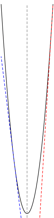
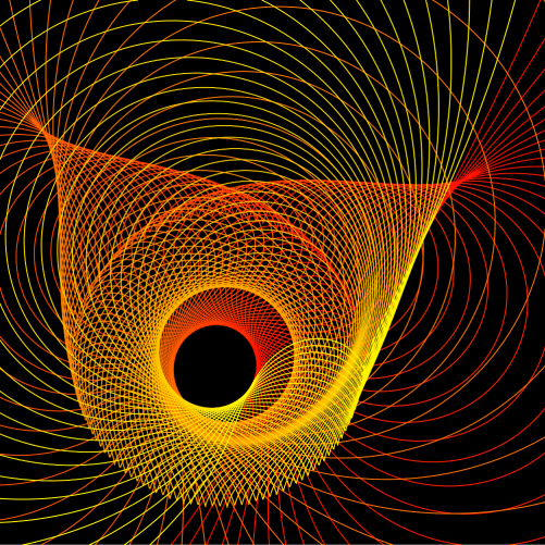
So what you see in the above image is several copies of the parabola y=x^2 inverted about a series of equally spaced points along the line segment with endpoints (1/2,-1/2) and (3/2,1/2).  This might seem a little arbitrary, but it takes quite a bit of experimentation to find a set of points to invert about in order to create an aesthetically pleasing image.

Of course there is another perspective on accomplishing the same task — just shift the parabolas first, invert about the origin, and then shift back.  This is geometrically equivalent (and the algebra is the same); it just depends on how you want to look at it.

Here is another image creating by inverting the parabola y=x^2 about points which lie on a circle.

2017-07-18Inversion1v2

And while we’re on the subject of inverting parabolas, let’s take a moment to discuss the cardioid example we looked at in our last conversation about inversion:

Cardioid2

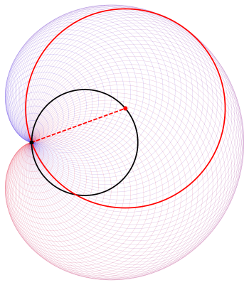
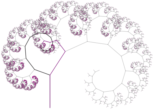
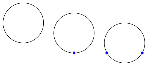
To prove that this construction of circles actually yields a cardioid, the trick is to take the inverse of a parabola about its focus.  If you do this, the tangent lines of the parabola will then invert to circles tangent to a cardioid.  I won’t go into all the details here, but I’ll outline how the proof goes using the following diagram.

Day104ParabolaProperty

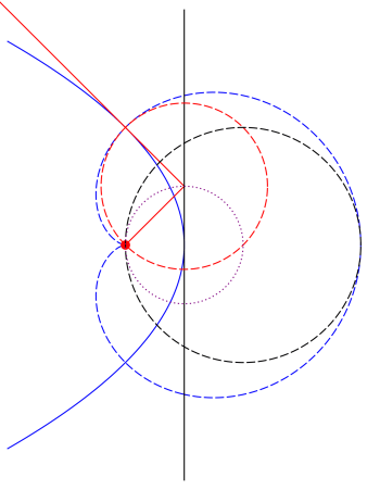
Draw a line (shown in black) tangent to the blue parabola at its vertex; the inverse curves are shown in the same color, but dashed.  Note that the black circle must be tangent to the blue cardioid since the inverse black line is tangent to the inverse parabola.

The small red disk is the focus of the parabola.  Key to the proof is the property of the parabola that if you draw a line from the focus to a point on the black line and then bounce off at a right angle (the red lines), the resulting line is tangent to the parabola.  So the inverse of this line — the red dashed circle — must be tangent to the cardioid.

Since perpendicularity is preserved and the line from the focus inverts to itself (since we’re inverting about the focus), the red circle must be perpendicular to this line — meaning that the line from the focus in fact contains a diameter, and hence the center, of the red circle.  Then using properties of circles, you can show that all centers of circles formed in this way lie on a circle (shown dotted in purple) which is half the size of the black circle.  I’ll leave the details to you….

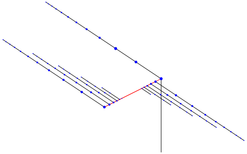
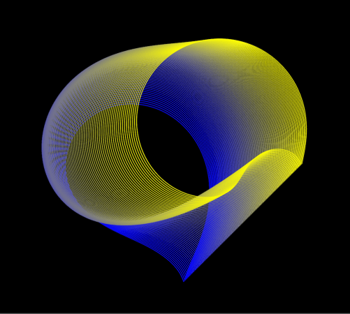
Finally, I’d like to show a few examples of using the other conic sections.  Here is an image with 80 inversions of an ellipse around centers which lie on a line segment.

2017-07-22Inversion1v2

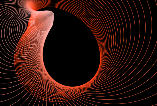
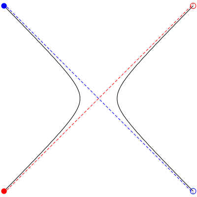
And here is an example of 100 hyperbolas inverted around centers which lie on a line segment.  Since the tails of the branches of a hyperbola all go to infinity, they all meet at the same point when inverted.

2017-07-22Inversion2v2

So now you know how to work with geometrical inversion from an algebraic standpoint.  I hope seeing some of the fascinating images you can create will inspire you to try creating some yourself!

Imagifractalous! 7: Fractal Binary Trees IV

Bridges 2017 is next week in Waterloo, Ontario, Canada!  We’re all looking forward to it…Nick and his parents are also going, and I’ll get to see a lot of new friends I met last year in Finland.

In preparation, I’ve been creating a portfolio of binary and ternary trees.  I’ve been coloring and highlighting the branches to make them easier to understand, so I thought I’d take the opportunity to share several of them.  Mathematics just as it’s happening….

Here is an example of what I’m talking about.

2017-07-20-0is11v1

Recall that we’re generalizing the idea of “left” and “right” branches of a binary tree — rather that just rotating left or right (and possibly scaling), we’re allowing any affine transformation to correspond to “left” and “right.”  In order to avoid any confusion, let’s refer to the transformations as “0” and “1.”

In the tree above, the 0 branches are shown in black, and the 1 branches in red.  Notice that sometimes, the 0 branches seem to go to the right, other times, to the left.  This is a common occurrence when you allow the branching to be determined by more general transformations.

Here, you’ll notice that 0 and 11 take you to the same place — beginning with the trunk (the vertical black line at the right), if you follow one black branch, you’ll end up at the same blue node as you would if you followed two red branches.  In fact, no matter what blue node you start at, following one black branch will always take you to the same place as following two red branches.

Here is not the place to go into too many details, but let me give you the gist of what we’re studying.  If you denote the transformation which generates the black branches by B_0 
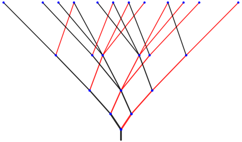
and that which generate the red branches by B_1, 
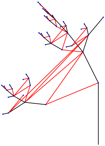
you will observe behavior like that in the above tree if

B_0=B_1+B_1^2.

Right now, most of the work I’m doing revolves around saying that I want to generate a tree with a certain property (like 0 and 11 going to the same node), and then solving the corresponding matrix equation to find interesting examples of trees with this property.  Usually the linear algebra involved is fairly complicated — feel free to comment if you’d like to know more.  As I said, this blog is not the place for all the details….

Below is another interesting example.

2017-07-20-0is00v2.png

In this tree, 0 and 00 go to the same node.  What this means in terms of branching is that there can never be two consecutive black branches (again, 0 is black and 1 is red) — taking the additional 0 branch leaves you in exactly the same place.

Note that for this property to hold, there is no restriction on what the 1 transformation can be.  Above, the transformation B_1 
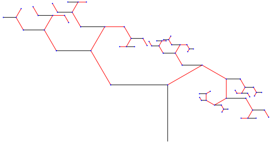
is a scaled rotation by 60°.  This is what produces the spirals of red branches emanating from the nodes of the tree.

2017-07-20-0is01v1.png

In this example, 0 and 01 go to the same node (0 is black, 1 is red).  Implications for the tree are that the red branches zigzag back and forth, getting shorter with each iteration.  Moreover, there aren’t any red branches drawn after a black branch (except the first time, off the end of the trunk of the tree).  This is because 01 — taking a red branch after a black branch — takes you to the same place as 0, which is taking a black branch.  In other words, the red branch doesn’t take you any further.

2017-06-27-01is10.png

Here, 01 and 10 take you to the same node (again, 0 is black and 1 is red).  This is easy to see — there are many quadrilaterals in the tree formed by alternating red and black branches.  In addition, the iterations of this tree move progressively higher each time — so, for example, all the nodes at the top are at a depth of 4.

If you look at the number of new nodes at each level, you get a sequence which begins

2, 3, 6, 12, 24, 48, 96, 192, 384, 768, ….

After the second level, it seems that the number of new nodes doubles with each iteration.  I say “seems” since it is generally very difficult to prove that such a relationship continues up arbitrarily many levels.  Although it is easy to find the sequence of numbers of nodes for any tree using Mathematica, I have rigorous proofs of correctness for only three cases so far.

What makes the proofs so difficult?  The following tree is another example of a case where 01 and 10 go to the same node.

2017-06-25-01is10v1

But the sequence of new nodes at each level is just 2, 3, 4, 5, 6, ….  (This is one case I’ve rigorously proved.)  The transformations B_0 and B_1 used to make this tree, in addition to forcing 01 and 10 to go to the same node, also have additional properties which force any two strings of the same length with the same number of 0’s (and therefore the same number of 1’s as well) to go to the same node.  So to prove the sequence of nodes in the previous case is 2, 3, 6, 12, 24, 48, …, you need to say which strings take you to the same nodes, and prove that this pattern continues no matter how far you go up — and that there are no “surprise” coincidences of other nodes as you proceed.

It is also possible to look at infinite strings going to the same node, as shown below.  The linear algebra gets quite a bit more involved in these cases.

2017-07-02infp1q1.png

Here, 0 and 1 do in fact correspond to going left and right, respectively.  The thicker black path corresponds to the string 011111…, that is, going left once, and then going to the right infinitely often, creating the spiral you see above.  The thicker green path corresponds to alternating 10101010… infinitely often, creating a zigzag path which approaches exactly the same point as the black spiral does.

Here is another example, where the spiral 011111… (in black) approaches the same point as the infinite zigzag 100100100100… (in purple).

2017-07-02infp1q2.png

These are some of my favorite examples.  But I should remark that once you know how to mathematically find transformations which produce trees with a desired property, it takes a lot of fiddling around to find aesthetically pleasing examples.

I hope these examples give you a better idea of the nature of our research.  I’ll update you on Bridges when I get back, and let you know about any interesting comments other participants make about our trees.  I leave on Wednesday, and will post pictures daily on my Twitter @cre8math if you’d like a daily dose of mathematical art!

More on: What is…Projective Geometry?

This week, I thought I’d go a little deeper into the subject of projective geometry (feel free to reread last week’s post for a refresher).  Why? I think this is a good opportunity to discuss the idea of an algebraic model of a geometry.  Certainly using Cartesian coordinates in the Euclidean plane makes many geometrical problems easier to approach.

So what would a coordinate system in projective geometry look like?  The most commonly used system is homogeneous coordinates.  Let’s see how they work.

The difficulty with adding the line at infinity is that we need infinitely many points in addition to those already in the plane.  Perhaps you might imagine that adding an “infinite” coordinate might do the trick, but there is an alternative — and algebraically simpler — approach.

First, think of the Euclidean plane as being the plane z = 1 in three-dimensional Cartesian coordinates, so that every Euclidean point (xy) is given homogeneous coordinates (xy, 1).  But we don’t want to make the z-coordinate special — we want all the homogeneous coordinates to have similar interpretations.  We accomplish this by giving each point infinitely many names — specifically, for any k ≠ 0, the coordinates (kxkyk) describe the same point as (xy, 1).  Geometrically, you might think of this as saying that the line through  (xy, 1) (except the origin) is, in some sense, the point (xy, 1).

So if z ≠ 0, the point (xyz) in homogeneous coordinates is another name for the Euclidean point (x/zy/z).  But why would you want to do this?

The punch line is that we can now use z = 0 to indicate that a point is on the line at infinity!  We still keep the convention that if k ≠ 0, the homogeneous coordinates (kxky, 0) describe the same point as (xy, 0), as long as x and y are not both 0.

So our system of homogenous coordinates contains all points (xyz) such that not all three coordinates are 0.  Any point with z ≠ 0 corresponds to a Euclidean point, and any point with z = 0 corresponds to a point on the line at infinity.

Is it really worth all this trouble?  There are many interesting features of such a coordinate system — and I’d like to mention a few of them here, omitting the proofs.  There are many resources online that include all the details — one example is the classic Projective Geometry by Veblen and Young available free as an ebook.

Let’s start be looking at equations of lines in projective geometry.  In the Cartesian plane, we may represent a line in the form Ax + By + C = 0, where A, B, and C are not all zero.  In the projective plane, a line has the form form Ax + By + Cz = 0, where A, B, and C are not all zero.  Nice, isn’t it?  This form is also consistent with our system of having many names for a point:  if Ax + By + Cz = 0 and k ≠ 0, then also A(kx) + B(ky) + C(kz) = 0 as well. So no problems there.

But the really neat aspect of this representation is how you can use linear algebra in three dimensions to solve many problems in projective geometry.  This isn’t a post about linear algebra — so I’ll limit myself to just one example.  But in case you do know something about linear algebra, I think you should see how it can be used in projective geometry when homogeneous coordinate are used.

We’ll consider the problem of finding the intersection of two lines, say Ax + By + Cz = 0 and Dx + Ey + Fz = 0.  The form of these expressions should remind you of taking the dot product, so that we can rewrite these expressions as

(A,B,C)\cdot(x,y,z)=(D,E,F)\cdot(x,y,z)=0.

Interpreting these coordinates and coefficients as vectors in three-dimensional space, we observe that the common point (xyz) is simultaneously perpendicular to both (A, B, C) and (D, E, F), since both dot products are zero.  So (xyz) can be found using the cross-product

(x,y,z)=(A,B,C)\times(D,E,F).

Very nice!  Again, there are many such examples, but this is not the place to discuss them….

This algebraic model also suggests another geometric model for the projective plane besides adding a line at infinity to the Euclidean plane.  Begin with the surface of a sphere centered at the origin in three-dimensional Cartesian space, and observe that opposite points on the sphere have homogeneous coordinates that are different names for the same point in the projective plane.

So, in some sense, we have exactly twice as many points as we need — so we identify opposite points on this sphere, so that they are in fact the same point.  (You might recall a similar discussion about points in the post on spherical geometry.)  Thinking about it in another way, we might just consider the top hemisphere of the sphere with only half of the equator, including just one of the endpoints of the semicircle.

And while this model is fairly simple geometrically, it is important to point out that this does not mean that the projective plane lies inside three-dimensional space.  Once we have our hemisphere and semicircle, we have to think about it without any of the surrounding space.  This is not easy to do, but this type of thinking is necessary all the time when studying differential geometry, a topic for another time….

One last benefit to using homogenous coordinates:  it can easily be abstracted to any number of dimensions.  Do you want a projective space?  Just add a plane at infinity to three-dimensional Euclidean space!  Coordinates are easy — all points (x, y, z, w), with not all coordinates equal to 0.  When w ≠ 0, the point (x, y, z, w) corresponds to the Euclidean point (x/w, y/w, z/w), and when w = 0, the point is on the plane at infinity.

And clearly, there would be no need to stop at three dimensions — it is just as easy to create a projective space of four or more dimensions.

Finding a workable system of coordinates for a particular geometry is not always a simple matter — but finding a system that allows problems to be solved easily is often a key step to studying any type of geometry.  I hope this gives you some insight to yet another aspect of the diverse universe of so many different Geometries….

What is…Projective Geometry?

The last type of geometry I discussed was inversive geometry, which is obtained by adding a point at infinity to the Euclidean plane.  Recall that as long as we had a consistent, useful model of this extended plane, it made perfect sense to define this new type of geometry.

Today, we’re going to add a line at infinity — creating what is called a projective geometry.  There are in fact many different types of projective geometries, but let’s just try to understand one at a time….

You might remember one important property of ω, the point at infinity in inversive geometry:  it was on every unbounded curve, and in particular, on every line. We need to be a bit more specific with our projective geometry, in the following sense.  Every line will intersect the line at infinity — denoted by λ — but not every line will intersect at the same point.

Consider all lines with some given slope m.  We then add one point to λ which lies on these lines, but no other lines.  In other words, each point on λ corresponds to an infinite family of parallel Euclidean lines — since now, with the addition of λ, there are no parallel lines in the projective plane.  The point at which two parallel (in the Euclidean sense) lines intersect is determined by their slope.

How does this differ from inversive geometry?  Well, in inversive geometry, if two lines had different slopes, they intersected in two points:  the usual finite point of intersection you learned about in algebra class, as well as ω.  But in projective geometry, two lines with different slopes intersect in only one point, since they intersect the line at infinity in two different points.

What this means is that any two distinct lines always intersect in exactly one point.  See the difference?  Parallel lines (in the Euclidean sense) intersect in a point on λ, and nonparallel (in the Euclidean sense) lines intersect in the same point they did in Euclidean geometry.

Now let’s look at the dual question (recall the discussion of duality, an important concept in spherical geometry):  what about a line between two points?  Two finite points generate a line, as usual.  If one point is finite and one lies on λ, the line generated is that line through the finite point with the slope corresponding to the point on λ.  And if both points are infinite, then the line through them is just λ.

Thus we have the following duality:  two distinct lines determine a unique point, and two distinct points determine a unique line.  Again, duality is an extremely powerful concept in geometry, so the fact that points and lines are dual concepts really is a legitimate justification for thinking about projective geometry.

Projective plane geometry is a broad subject — but some of my favorite objects to look at in projective geometry are the conic sections:  ellipses, parabolas, and hyperbolas.  This is because from the point of view of projective geometry, they are, in a sense which we’ll look at right now, all the same.

This sounds odd at first reading, but follow along.  The first question we need to consider is what points on λ lie on unbounded curves.  For lines, it’s easy — it’s just the point on λ corresponding to the slope of the line.

Now what about a parabola?parabola

You can see from the image that as points on the parabola move further away from its vertex, the tangents have slopes of ever-increasing magnitude.  Determining the precise slopes is an easy exercise in calculus — but what is important is that the tangent lines approach, in slope, the axis of the parabola.  In this case the axis is vertical, but of course the parabola may be rotated.

What this means is that the parabola intersects the line at infinity in the point corresponding to the slope of its axis.  Again, the tangent lines on either side approach this slope, but from two directions — from above and from below.

Now hold this thought while we look at a hyperbola.

hyperbola

Let’s see how we travel along the hyperbola.  As we move to the upper right toward the open red circle, we are moving closer to the red dashed asymptote — meaning we approach the point on λ corresponding to the slope of the red asymptote.  But here is where it becomes interesting:  as we cross the line at infinity, we come back along the asymptote toward the filled red circle on the other branch of the hyperbola!

Then we continue moving along the left branch, getting continually closer to the blue asymptote, approaching that point on λ corresponding to the slope of the blue asymptote as we pass through the blue filled circle.  Then we cross the line at infinity again, and jump to the right branch of the hyperbola toward the open blue circle.

Can you see what this means?  In projective geometry, a hyperbola does not have two separate branches.  Adding the line at infinity allows us a means to jump between the two branches.

Let’s look at these scenarios from a slightly different perspective.  Suppose that somehow, we can actually draw the line at infinity.  It’s the blue dashed line in the figure below.  Easy.

conics

Can you see where we’re going with this?  The left circle represents an ellipse, since it is a bounded curve and cannot intersect λ.  The middle circle represents a parabola — it’s a curve which intersects the line at infinity at exactly one point, and so is actually tangent to λ.  The right circle represents a hyperbola, since it intersects the line at infinity at two points.  It may look strange from this perspective, but this right circle really does represent the hyperbola illustrated above.

To summarize:  if a conic does not intersect the line at infinity, we call it a Euclidean ellipse, if it is tangent to λ, we call it a Euclidean parabola, and if it intersects λ in two points, we call it a Euclidean hyperbola.

Because you see, in projective geometry, there is no distinguished line.  Every line is just like any other.  So, in some sense, these is just one conic section in projective geometry!

What we have looked at today is what would be called an embedding of the Euclidean plane in the projective plane.  We saw how we could just add a line at infinity with certain properties, and our plane would behave “projectively.”  But from the perspective of projective geometry, you’ve just got conic sections and lines, with possibly 0, 1, or 2 intersection points as illustrated above.  A little mind-blowing, but absolutely true.

Of course we’ve only been able to scratch the surface of this really amazing geometrical world today.  Hopefully you will be inspired to learn a little bit more about it….

100 Posts!

Can you believe it?  I have been waiting to be able to finally tag “Day1xx”, and that day is finally here!

I could say something momentous on this occasion.  But I’m not sure that’s really necessary — you can imagine that keeping a blog running for 100 weeks with (hopefully!) interesting posts on mathematics, creativity, and art is momentous emough.

But I have been running into a problem:  my blog is getting harder to search.  For example, I just got five pages of results by searching for “fractal”!  So I thought I’d put together an index of all my blog posts, organized by category.

I hope this is of use to newer followers — you might like certain topics better than others, and this way you can easily look at older posts related to the ones you like.

The category a post is listed under is what I consider its primary category — but rarely does a single post only address on topic.  But surely this index is a step in the right direction.

And lastly, I would like to thank all my followers for encouraging to keep me going.  I get an email every time someone likes or comments — and I appreciate each one. Thanks again!

A.  Introduction

  1. Day001, What Is Mathematics?

B.  Mathematical and Digital Art

  1. Day002, Josef Albers and Interaction of Color.
  2. Day011, Evaporation I.
  3. Day012, Evaporation II.
  4. Day015, Geometrical Dissections II: Four to One.
  5. Day022, Envelopes III:  Art and Randomness
  6. Day029, The Joy of Ink I.
  7. Day030, The Joy of Ink II.
  8. Day054, Color I: Opacity and Josef Albers.
  9. Day055, Color II: Opacity and Josef Albers.

C.  Mathematical Puzzles

  1. Day003, CrossNumber Puzzles.
  2. Day005, Cryptarithms.
  3. Day010, ColorSlide Puzzles.
  4. Day018, Roman Numeral Puzzles.
  5. Day024, Logic Puzzles I.
  6. Day025, Logic Puzzles II.
  7. Day031, Number Searches I.
  8. Day032, Number Searches II.
  9. Day109, Beguiling Games I:  Nic-Nac-No.
  10. Day114, Beguiling Games II:  Nuh-Uh!
  11. Day119, Beguiling Games III:  Splotch!
  12. Day122, Knights and Rogues.
  13. Day125, Beguiling Games IV:  Scruffle.
  14. Day132, More CrossNumber Puzzles.

D.  Two-Dimensional Geometry

  1. Day004, Hexominoes and Cube Nets.
  2. Day014, Geometrical Dissections I.
  3. Day020, Envelopes I.
  4. Day021, Envelopes II:  Making Spirals.
  5. Day074, The Ravioli Equation.
  6. Day106, Polygons.
  7. Day118, Geometrical Dissections III:  Octagons and Dodecagons.

E.  Pedagogy

  1. Day006, Day163 (reprise), The Problem with Calculus Textbooks.
  2. Day013, Writing Original Problems.
  3. Day023Day093 (reprise), The Problem with Grades.
  4. Day026, On Grading.
  5. Day028, International Dodecahedron Day 2016!
  6. Day158, Teaching Three-Dimensional Geometry, I.
  7. Day160, Teaching Three-Dimensional Geometry, II.
  8. Day161, Teaching Three-Dimensional Geometry, III.
  9. Day164, On Assessment, I.
  10. Day165, On Assessment, II.
  11. Day166, On Assessment, III.
  12. Day167, On Assessment, IV.
  13. Day168, On Assessment, V.

F.  Koch Curves and Related Topics

  1. Day007, Creating Fractals.
  2. Day008, Creating Fractals II: Recursion vs. Iteration.
  3. Day009, Creating Fractals III: Making Your Own.
  4. Day027, Creating Fractals IV:  Results!
  5. Day033, New Koch Snowflakes.
  6. Day062, Koch Curves and Canopies.
  7. Day065, p-adic Numbers I: When Big is Small.
  8. Day067, p-adic Numbers II: When Big is Small.

G.  Essays

  1. Day016, On Mathematical Creativity I.
  2. Day017, On Mathematical Creativity II.
  3. Day019, Writing a Math Blog.

H.  Iterated Function Systems

  1. Day034, Creating Fractals V:  Iterated Function Systems I.
  2. Day035, Creating Fractals VI:  Iterated Function Systems II.
  3. Day036, Creating Fractals VII:  Iterated Function Systems III.

I.  Programming and Coding

  1. Day037, Creating Fractals VIII:  PostScript Programming.
  2. Day058, On Coding I.
  3. Day060, On Coding II: LISP.
  4. Day064, On Coding III: LISP to Mathematica.
  5. Day068, On Coding IV: Mathematica.
  6. Day075, On Coding V: Postscript.
  7. Day078, On Coding VI: HTML.
  8. Day082, On Coding VII: LaTeX I.
  9. Day085, On Coding VIII: LaTeX II.
  10. Day092, On Coding IX: Computer Graphics I.
  11. Day099, On Coding X: Computer Graphics II.
  12. Day107, On Coding XI: Computer Graphics III, POV-Ray.
  13. Day117, On Coding XII:  Python.
  14. Day121, On Coding XIII:  Retrospective.

J.  Mathematics and Art Conferences

  1. Day038, Bridges:  Mathematics and Art I.
  2. Day049, Bridges:  Mathematics and Art II.
  3. Day050, Vienna!  (Symmetry Conference 2016).
  4. Day053, Bridges: Mathematics and Art III. Jyvaskyla, Finland!
  5. Day083, Art Exhibition: Golden Section 2017.
  6. Day105, Bridges 2017 in Waterloo, Canada!
  7. Day134, Art Exhibition: Golden Section 2018.
  8. Day169, Jagodina, Serbia:  2018.

K.  Processing

  1. Day039, Making Movies with Processing I.
  2. Day040, Making Movies with Processing II.
  3. Day041, Making Movies with Processing III.
  4. Day042, Making Movies with Processing IV.
  5. Day043, Making Movies with Processing V.
  6. Day044, Making Movies with Processing VI.
  7. Day108, To Processing I.
  8. Day110, Using Processing for the First Time.
  9. Day113, Creating Animated GIFs in Processing.

L.  Mathematics and Digital Art Course

  1. Day045, Mathematics and Digital Art I.
  2. Day046, Mathematics and Digital Art II.
  3. Day047, Mathematics and Digital Art III.
  4. Day048, Mathematics and Digital Art IV.
  5. Day057, Digital Art I: End of Week 2 (Fall 2016).
  6. Day059, Digital Art II: End of Week 4 (Fall 2016).
  7. Day061, Digital Art III: End of Week 6 (Fall 2016).
  8. Day063, Digital Art IV: End of Week 8 (Fall 2016).
  9. Day066, Digital Art V: End of Week 11 (Fall 2016).
  10. Day069, Digital Art VI: End of Week 14 (Fall 2016).
  11. Day071, Digital Art VII: Final Projects! (Fall 2016).
  12. Day072, Digital Art VIII: The End (Fall 2016).
  13. Day081, Mathematics and Digital Art: Update 1 (Spring 2017).
  14. Day086, Mathematics and Digital Art: Update 2 (Spring 2017).
  15. Day090, Mathematics and Digital Art: Update 3 (Spring 2017).
  16. Day094, Mathematics and Digital Art: Final Update (Spring 2017).
  17. Day112, Mathematics and Digital Art: Update 1 (Fall 2017).
  18. Day115, Mathematics and Digital Art: Update 2 (Fall 2017).
  19. Day123, Mathematics and Digital Art: Final Update (Fall 2017).

M.  Guest Bloggers

  1. Day051, Guest Blogger:  Geoffrey Owen Miller, I.
  2. Day052, Guest Blogger:  Geoffrey Owen Miller, II.
  3. Day096, Guest Blogger: Percival Q. Plumtwiddle, I.
  4. Day097, Guest Blogger: Percival Q. Plumtwiddle, II.
  5. Day154, Transforming Mathematics Education:  BAMAS, X.
  6. Day155, Guest Blogger:  Scott Kim, II.
  7. Day156, Guest Blogger:  Scott Kim, III.
  8. Day157, Guest Blogger:  Scott Kim, IV.

N.  Milestones

  1. Day056, Celebrating One Year!

O.  Imagifractalous!

  1. Day070, Imagifractalous! 1: How it all began.
  2. Day073, Imagifractalous! 2: p-adic sequences.
  3. Day077, Imagifractalous! 3: Fractal Binary Trees.
  4. Day087, Imagifractalous! 4: Fractal Binary Trees II.
  5. Day088, Imagifractalous! 5: Fractal Binary Trees III.
  6. Day089, Imagifractalous! 6: Imagifractalous!
  7. Day103, Imagifractalous! 7: Fractal Binary Trees IV.

P.  What is a Geometry?

  1. Day076, What is a Geometry?
  2. Day079, What is…Taxicab Geometry?
  3. Day084, What is…Spherical Geometry?
  4. Day091, What is…Inversive Geometry?
  5. Day095, More on: What is…Inversive Geometry?
  6. Day101, What is…Projective Geometry?
  7. Day102, More on:  What is…Projective Geometry?
  8. Day104, Still more on:  What is…Inversive Geometry?
  9. Day152, What is….A Polygon?

Q.  Miscellaneous Mathematics

  1. Day080, A New Cantor Set?
  2. Day098, The One Four Conjecture.
  3. Day147, Pythagorean Triples.
  4. Day153, Circle Geometry.

R.  Bay Area Mathematical Artists

  1. Day111, Bay Area Mathematical Artists, I.
  2. Day116, Bay Area Mathematical Artists, II.
  3. Day120, Bay Area Mathematical Artists, III.
  4. Day124, Bay Area Mathematical Artists, IV.
  5. Day131, Bay Area Mathematical Artists, V.
  6. Day135, Bay Area Mathematical Artists, VI.
  7. Day140, Bay Area Mathematical Artists, VII.
  8. Day144, Bay Area Mathematical Artists, VIII.
  9. Day149, Still Moving On (and BAMAS IX)….
  10. Day154, Transforming Mathematics Education:  BAMAS, X.
  11. Day159, Bay Area Mathematical Artists Seminars, XI.

S.  In Memory of Fr. Magnus J. Wenninger, O.S.B.

  1. Day 126, Fr. Magnus Wenninger, O.S.B, I.
  2. Day 127, Fr. Magnus Wenninger, O.S.B, II.
  3. Day 128, Fr. Magnus Wenninger, O.S.B, III.
  4. Day 129, Fr. Magnus Wenninger, O.S.B, IV.
  5. Day 130, Fr. Magnus Wenninger, O.S.B, V.

T.  The Puzzle Archives.

  1. Day133, The Puzzle Archives, I.
  2. Day136, The Puzzle Archives, II.

U.  Calculus

  1. Day006, The Problem with Calculus Textbooks.
  2. Day137, The Geometry of Polynomials.
  3. Day138, Calculus:  Linear Approximations, I.
  4. Day139, Calculus:  Linear Approximations, II.
  5. Day141, Calculus:  The Geometry of Polynomials, II.
  6. Day142, Calculus:  Hyperbolic Trigonometry, I.
  7. Day143, Calculus:  Hyperbolic Trigonometry, II.
  8. Day145, Calculus:  Hyperbolic Trigonometry, III.
  9. Day146, Calculus:  Hyperbolic Trigonometry, IV.
  10. Day150, Calculus VII:  Approximations.  [Not sure how the numbering got off….]
  11. Day151, Calculus VIII:  Miscellaneous Problems, I.

V.  Truly Miscellaneous….

  1. Day148, Moving Out and Moving On….
  2. Day149, Still Moving On (and BAMAS IX)….

W.  Polyhedra

  1. Day162, Enumerating the Platonic Solids.
  2. Day174, My Polyhedra Textbook, I.
  3. Day175, My Polyhedra Textbook, II.

X.  Four-Dimensional Geometry

  1. Day170, The Fourth Dimension, I.
  2. Day171, The Fourth Dimension, II.
  3. Day172, The Fourth Dimension, III.
  4. Day173, The Fourth Dimension, IV.