Digital Art VI: End of Week 14

The last three weeks have been very intense!  The main focus has been on laboratory work, both with Processing and Final Projects.

Week 12 began with another round of Presentations on papers from past Bridges conferences.  This proved to be successful again — with topics ranging from geometrical furniture to zippergons to maps of Thomas More’s Utopia.  We all learned something new!

The time not spent on Presentations that week was devoted to working on projects.  Students were finding their stride, and their ideas were really beginning to take shape.

Two students were interested in image processing, so Nick has been working with them.  The initial problem was that doing anything in Sage involving image processing was just too slow — you’re code is essentially sent to a remote server, executed, and the results sent back.  Since we’re using the free version, this means performance is unpredictable and far too slow for computation-heavy tasks.

So Nick helped with installing Python, finding image processing packages, etc.  This process always takes a lot longer than you imagine, but eventually all issues were resolved.

While Nick was working on image processing, I was helping others.  One student was really interested in using L-systems — one of my favorite geometrical topics recently!   But all my work with Thomas involved code written in Postscript and Mathematica.  Which meant I had to rewrite it in Python.

This proved to be quite a bit trickier than I thought.  The student was looking at The Algorithmic Beauty of Plants, and was interested in modeling increasingly complex L-systems.  First, the simplest type, like that used to generate the Koch curve.  Next came bracketed L-systems, and then bracketed L-systems with multiple rules.  I did finally get all these to work; I intend to clean up the code and share it in a future post.

Week 13 was devoted entirely to Processing and project work.  I started the week with introducing a few new ideas.  What really inspired the class were the mouseX and the mouseY variables.  When your mouse is in screen space, the mouseX and mouseY variables contain the location of your mouse.  So you can put an object where the mouse is, or have the x-coordinate of the mouse in some way determine the color or the size of the object.  The possibilities are virtually endless.

Here’s a sample movie made with this technique.

Since the code is just a few lines long, it won’t take long to explain.  Here is the complete program:

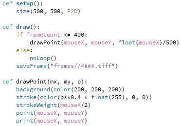
The drawPoint function will draw a point centered at the position of the mouse.  But in addition to those coordinates, the function takes an addition argument:  float(mouseX)/500.  This argument is 0 at the left edge of the screen, and 1 at the right edge.  (Recall the need for “float,” since otherwise Python will perform integer division and give 0 for any number less than 500.)

So the stroke command uses the parameter p to determine how much red is in the color specification.  When p is 0, there is no red, so the dot is black.  And when p is 1, the dot is red.  I used “p**0.4” as an illustration that interpolation need not be linear — the exponent of p determines how quickly or slowly the dot gets brighter as you move the mouse to the right.  Of course the dot also gets larger as you move your mouse to the right, as is clear by the strokeWeight function call.

I showed this example as I introduced the movie project.  Their assignment was to make a movie — anything they wanted to try.  The complete prompt is given on Day 34 of the course website, but I’ll give the gist of it here.  The main goal was to have students use linear interpolation in at least four different ways in their movie.  Of course they could use nonlinear interpolation if they wanted to, but it wasn’t required.

There was no length requirement — it’s easy to make a movie longer by adding more frames.  Just be creative!  Interpolation is a very useful tool in making movies and animations, and has a mathematical basis as well.  So I wanted that to be the focus of the project.  I also had them write a brief narrative about their use of interpolation.

This is Andrew’s movie.  You can clearly see the use of interpolation here in different ways.  It was also nice to see the use of trigonometry to calculate the centers of the dots.

 

Ella was interested in L-systems, and so Nick spent some time working with her on Python code during his weekly office hours.  Here is what she created.

 

Lucas wanted to use some interaction with the mouse, and he also had the idea of the sun setting as you moved the mouse down the screen.  Watch how the fractal clouds move with the location of the mouse as well.

 

So you can see how varied the use of interpolation was!  The students really enjoyed having control over the possible special effects, and created a wide range of interesting features in their movies.

That takes us to Week 14.  On Monday, we had a guest speaker come in, Chamberlain Fong.  I met him in Finland at Bridges this summer, only to find out he lives the next neighborhood over in San Francisco!  He gave a very interesting talk about taking pictures with a spherical or hemispherical camera lens, and the issues involved in printing the pictures.

The problem is essentially the same as creating a map of the globe — making a sphere flat.  There will always be distortion, but you have some control over what type of distortion.  You can keep angles the same, or areas the same — or some combination of the two.  And as these cameras keep getting cheaper, there will be a growing interest in making your spherical photos look realistic.

And although we had class on Wednesday, some students had already left for Thanksgiving Break.  So Nick and I were available to help on an open lab day.  Most of the students actually showed up, and we had a productive day working on movies (which were due Wednesday) and projects.

The next (and final!) post on Mathematics and Digital Art will survey the students’ Final Projects, so stay tuned!