November 2015 – Creativity in Mathematics

Geometrical Dissections II: Four to One

This week, I’d like to discuss a piece of artwork which began as a geometrical dissection — I call it Four to One.

Day015FourToOneWeb

I thought it would be interesting to discuss the process of creating such a piece from beginning to end. The creative process is not really mystical, but because we so often only see the finished product, it may seem that way at times.

It all began about 15 years ago, when I was teaching the Honors Geometry course I mentioned in last week’s post. In Greg’s book Dissections Plane & Fancy, he takes a few chapters to discuss dissections from squares to other squares — frequently two different squares to one, or three to one. But there was very little about four-to-one dissections, so I thought I’d explore this avenue a bit more.

I can’t recall precisely how I arrived at the identity

$15^2+36^2+48^2+64^2=89^2.$

I might have written some for loops — but computers were not as fast back then…. Likely I used something like Lebesgue’s formula on p. 80 of Greg’s book, which gives a formula for creating three-to-one square dissections. Then if one of those squares could be written as a sum of two others, I’d have a four-to-one dissection. In particular, once I (might have!) found out that

$39^2+48^2+64^2=89^2,$

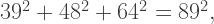
I could use the fact that $15^2+36^2=39^2$ (which is just a multiple of the Pythagorean triple $(5, 12, 13)$ ) to obtain the possibility of a four-to-one dissection described above.

Now this only suggested the puzzle, not the actual dissection itself. And there certainly is a dissection — at the very least, we can cut up all the squares into $1\times1$ unit squares and reassemble!

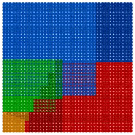
This is hardly an elegant solution; but I did come up with the following one:

Day015FourToOneGeometryWeb

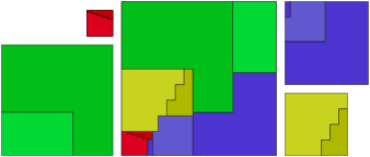
I liked it because each square was cut into just two or three pieces, which was particularly nice. Moreover, only one piece needed to be rotated. But even though the number of pieces is relatively small, there is still the possibility that a dissection may exist using fewer pieces.

Of course my original solution was sketched on a yellowing piece of graph paper — but what to do with it now?

My first attempt looked like this:

FourSquaresToOne

I was thinking of creating various pathways through the dissected squares so that when they were rearranged, the pathways would still line up. I abandoned this approach, however. I can’t remember exactly why, but the results didn’t appeal to me — and besides, the paths themselves actually had nothing to do with the dissection puzzle itself.

But then I had the thought — which was in fact a real challenge — can I communicate what’s happening with the dissection using only one square? In other words, could I depict the geometrical dissection by just showing the largest square without giving the viewer the four smaller squares? I think what might have moved me in this direction is that there was just no elegant way of putting all five squares together in a composition. There were just too many corners.

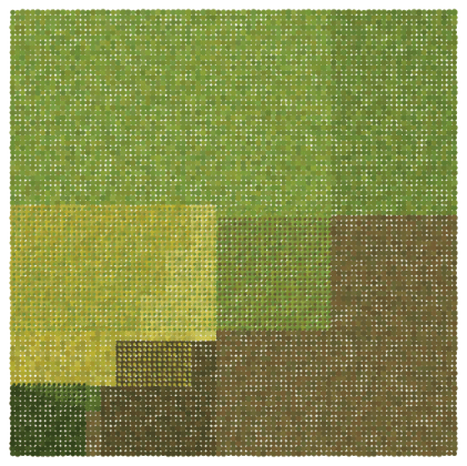
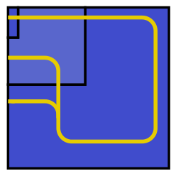
So I though of overlapping the smaller squares onto the largest square, as shown below (note: you’ll notice an error in the geometry, but as it was a draft I discarded, I didn’t bother to fix it):

Day015FourSquaresToOne2

Day015FourToOneGeometryWeb

Now if you look very carefully, you can find all the pieces of the dissected squares in the largest square. There is some overlap, of course — but smaller circles were overlaid on larger ones so colors from both circles could be seen. (I copied the original dissection again so it’s easier to compare. I used different colors as the images were created at different times, so watch out! )

I liked the idea — I felt I was getting somewhere. But I wasn’t happy with the colors. Now creating mathematical art makes you hungry — I can clearly recall driving to lunch while I was in the middle of this project, and I can even remember the road. It was Fall in Princeton, NJ, and the leaves had already turned color. No more oranges and reds — but lots of greens and yellows, as well as browns from the tree trunks. My color palette!

What intrigued me about the idea was the fact that I was working with a very abstract, almost purely mathematical problem — and here I was, thinking about using organic colors from nature, from my life experience.

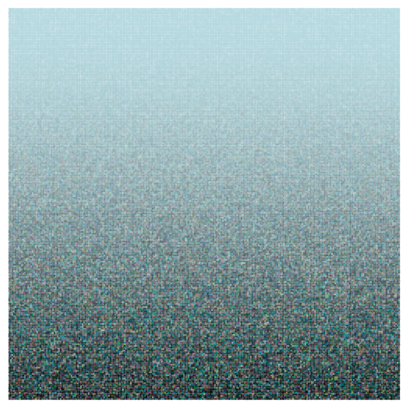
Now I had already been working with the ideas from Evaporation, and realized if I was using an organic palette, I couldn’t have the circles be regular, precise — and the colors couldn’t be pure either, just like you might find hundreds of shades of yellow in a Fall forest.

Day015FourToOneExcerptWeb

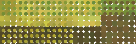
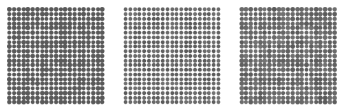
So, as shown in this close-up of Four to One, the colors were varied by using random numbers just as was done for Evaporation, but there were no extremes — each piece of each square had to be clearly recognizable if the dissection was to be clearly seen.

The sizes of the circles varied as well, helping to contribute to a natural texture. Here, you can clearly see how smaller circles were overlaid on larger circles for the two-color effect. The smaller circles, however, had only about one-fourth the area of the larger ones, so it was clear which color was dominant.

And there it is! The creative process is not magical, not mystical — in fact, much of the time it seems to consist of failed inspiration…. Consider yourself lucky if your first attempt turns out to be your last as well — but more often than not, creativity is an iterative process involving constant revision.

So my advice is to stick to it! Don’t worry if the first attempt isn’t what you imagine. Now I used Mathematica to create this image — and I’ve been programming in Mathematica for over twenty years. So I’m pretty good at taking an idea and implementing it fairly quickly. But if you’re relatively new to programming, you’ve got to be patient with your programming skills as well. I can tell you though — it’s worth it. Don’t let anyone else tell you any different….

Geometrical Dissections I

Closely related to the problem of tiling the plane with polygons is that of dissecting one geometrical object into pieces that can be rearranged to form another. The classic example is the following dissection of an equilateral triangle to a square, attributed to Henry Dudeney, 1907.

Day014TriToSquare

Note that the pieces are exactly the same in both polygons. It’s not hard to appreciate the beauty and elegance of this “geometrical artwork.” And it’s not hard to imagine a puzzle based on this dissection — give the puzzler these four pieces with instructions to make both a triangle and a square from the same pieces.

This led me, once upon a time, to construct an Honors Geometry course centered around geometrical dissections using Greg Frederickson’s wonderful Dissections Plane & Fancy.

But even “simple” dissections — involving triangles and squares — weren’t so easy to create. For example, the pieces divide the base of the equilateral triangle into lengths Day014formula and these are some of the easier calculations! I won’t say more about that here — but you can read all about this dissection and many others in Greg’s book.

So I was fascinated by geometrical dissections — but I needed a way to make the idea accessible to my students. I thought — what could you create just by experimenting with dissections on ordinary graph paper?

Well, I have been answering this question for over 15 years now. I’ll start with some introductory ideas in this post, but this is definitely not the last word on dissections!

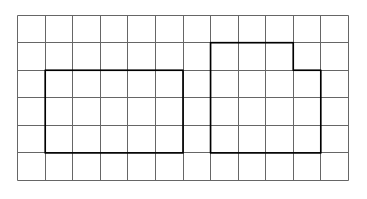
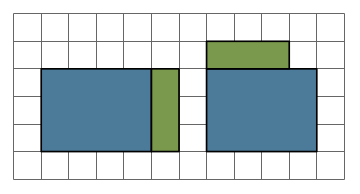
Let’s begin with the following puzzle. By cutting the rectangle along the grid lines, how many pieces are needed so you can also make the square with a corner missing? Day014Puzzle1A This seems like an easy puzzle to solve, as shown below. Day014Puzzle1B So yes, only two pieces are necessary — but one had to be rotated. Here is the question: can this puzzle be solved with just two pieces, but with neither piece rotated?

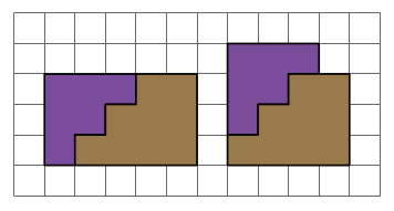
It turns out this is possible — but a solution requires a bit more creativity. Here is one way to do it: Day014Puzzle1C This is a solution technique commonly used in Dissections Plane & Fancy. Why bother? In the world of geometric dissections (and it is a growing universe, surely, as any internet search will show), finding a minimum number of pieces is the primary objective. But of all solutions with this minimum number of pieces, “nicer” solutions require rotating the fewest number of pieces. And rotating none at all is — in an aesthetic sense — “best.” It is also preferable not to turn pieces over, although sometimes this cannot be avoided for minimal solutions.

Another criterion for solutions might be whether they can be hinged or not, as Greg discusses extensively in Hinged Dissections: Swinging & Twisting. We won’t have time to explore this topic today.

Of course there is no reason you have to start with a rectangle, and also no reason why you need to restrict yourself to just one shape. The puzzle below shows how you can find a four-piece, rotation-invariant dissection from two smaller octagons to one larger octagon. Day014Puzzle2 It is important to note that the octagons here are not regular. A quick glance through Dissections Plane & Fancy will reveal that dissections involving regular polygons are generally rather difficult (as the initial triangle-to-square example amply shows).

Further, “two-to-one” dissections lend themselves nicely to a square grid, as the diagonal of a unit square has length square root of 2. Take a moment to study the octagon dissection again — paying particular attention to the side lengths — to see how this plays out. In the world of regular polygons, however, two-to-one dissections are in general quite difficult. Visit Gavin Theobald’s web page of two-to-one dissections to see some fascinating examples.

It is not hard to create dissection puzzles of your own — a pencil, eraser (!!!), and graph paper are all you need. What is difficult, however, is proving that you’ve found the fewest number of pieces. And when you have, proving that your dissection is unique. Uniqueness is virtually impossible to prove, but sometimes you can get a handle on minimality. For example, if the octagon dissection could be done in three pieces, one of the smaller octagons would have to be uncut. It’s not hard to see that there is no way of cutting the other smaller octagon into just two pieces to create the larger octagon.

What I enjoy about creating dissection puzzles is that there is not a single strategy you can use to solve them. You really need to use your imagination. Sometimes you might even surprise yourself by stumbling upon a really neat puzzle, like the one below.

Here, an 8 x 8 square with four holes (shown in black) can be dissected into three pieces to create a 6 x 10 rectangle, although one piece needs to be rotated. There is a simple elegance about this dissection which I find appealing. Day014Puzzle3

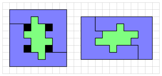
Another grid which lends itself to creating dissections is a grid of equilateral triangles. We won’t go into details here, but you can get the idea with the following dissection of an irregular dodecagon to an equilateral triangle in just five pieces. (The minimal dissection with regular polygons requires eight pieces.) Day014Puzzle4 I’ll leave you with two puzzles to think about. Of course, you can just make up your own. If you come with anything interesting, feel free to comment!

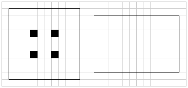
For this puzzle, my best solution is four pieces, without needing to rotate any pieces or turn any pieces over. (Black squares are holes.) Day014Puzzle5

For the last puzzle, my best solution is five pieces — but I had to turn over and rotate two of the pieces. Day014Puzzle6

A parting suggestion: when looking up dissections on the web, be sure to use the search words “geometrical dissections…..”

Writing Original Problems

How do students view mathematics?

Not surprisingly, many (if not most) students see mathematics as a set of known problems to be solved — changing a few numbers here and there, perhaps — but essentially, all of mathematics is known.

Mathematicians have rather the opposite view — we’re just scratching the surface. There is so much more underneath.

As I mentioned in my first post, mathematics is creative. What makes this difficult for students to appreciate is that the artistic medium is that of abstraction, and without a real understanding of abstraction in mathematics, the creative aspect is hard to see.

But there is a way to help students experience the creative side of doing mathematics — and that is by having them write their own Original Problems. I began thinking about this while I was teaching a course in problem solving at a magnet STEM high school — and being an avid problem writer myself, I imagined that having students write problems would help them solve problems. Whether this is true or not is difficult to determine. Regardless, an assignment was born….

What really got me interested in this assignment was the student comments at the end of the semester. One student wrote,

Anyone can write tedious, difficult problems that review core math subjects, but to write problems in a novel, challenging, and refreshing manner, one must be imaginative. I feel that this creative side of math is an often overlooked aspect of the field as many believe math to be an extremely black-and- white, rigid, and boring subject.

I was intrigued by the fact that even though students were not prompted to address creativity in writing their course evaluations, some spontaneously did so. As a teacher, I was delighted — an unanticipated side effect of an assignment designed for another purpose was somehow more significant to me than the intended outcome.

Fueled by this success, I introduced the assignment in an Honors Calculus section I taught, and students responded positively again. Then I incorporated writing Original Problems into a traditional calculus classroom, then precalculus, then algebra — and students kept getting it. Posing problems was no longer an assignment just for advanced students.

What does the assignment look like? I break it down into four sections. First, Motivation. Where did the problem come from? For some students, they might start looking in their textbook at interesting problems. For others, they take inspiration from their daily life. One calculus student said he came up with his problem because he dropped his backpack down the stairs and had to retrieve it — and he immediately thought of this as a displacement/velocity problem. Another student was doodling figure eights, and created a problem about ice skating on a figure-eight shaped rink. It is remarkable what students can create, given the opportunity!

Second, the Problem Statement. This is actually quite difficult for some students. And we teachers know the challenge of writing a test whose problems can be interpreted in only one way. Now that I’ve moved on from the STEM high school to teaching university again — and work with a different set of students — I now assign the Motivation and Problem Statement as a separate assignment. That way, I can give written and verbal feedback to students and help them craft a well-stated, manageable problem. This has been very helpful for the students, and the quality of their final submissions has improved.

Third is the Problem Solution. This is fairly self-explanatory, but a few comments are in order. I like to give students wide latitude in selecting a problem of interest to them — sometimes they want to challenge themselves with a difficult problem. In this case, a partial solution is fine. The point is to get them writing mathematics — and a partial solution to a difficult problem often involves more mathematics than a complete solution to a more routine problem.

Finally, there is the Reflection. I only ask for a few sentences or a paragraph — enough to give me a sense of how students are responding to the assignment. These can be very revealing, and you sometimes get students who really appreciate the assignment and understand its purpose. All four sections are to be included in the final submission.

You might be interested in a recent Original Problem prompt. This assignment is highly adaptable. I’ve had colleagues who wanted to narrow the focus because the assignment seemed to broad. Suggesting a specific application — such as the Pythagorean theorem — will give students a starting place. In my mind, the assignment is about creativity, writing, and self-determination. Let students choose a topic to create a scenario and write about it, and they start to get a handle on what creativity in mathematics is all about. There is no one way to accomplish this.

I should say a few words about grading these assignments. At their broadest, these assignments read like short essays. But they’re all different, so you can’t really develop a rhythm in the grading process. So Original Problems take more time to grade — this semester I’m just giving two assignments, so it’s more manageable. I do think it’s important to give at least two assignment, so students have a chance to improve. Generally, I’m more lenient when I grade the first assignment, since often this is the first time students will have encountered such an assignment.

To encourage creativity, I tell students that if they just do the assignment — and get their mathematics correct — they won’t earn lower than a B. I don’t want them worrying about grades (and we’re stuck with them for a while!), although some inevitably do. I rarely give a C, unless it’s evident a student waited until the last minute, or a student worked below their potential. I do believe that for an assignment like this, you should evaluate students relative to themselves, not their peers. More able students should be pushed — and frankly, most of them appreciate it when you do push them.

Many students really do begin to understand the creative aspect of mathematics after doing these assignments. They really do enjoy getting to choose their own problem — and though it is sometimes challenging to come up with a way for them to develop a particular idea, I rarely tell them to just choose another topic. I try to find some avenue they can pursue.

So I encourage you to give Original Problems a try! Let me know how it goes. For additional reading, you can find an article about writing Original Problems in Publication 10 on my website. There is also a discussion of several student problems in Chapter 6 of Mathematical Problem Posing. It really is time to have all students experience creativity in mathematics. This is one of the main purposes of writing this blog, after all.

Evaporation II

Last week, we began exploring the piece Evaporation. In particular, we looked at two aspects of the piece — randomness of both the colors and the sizes of the circles — and experimented with these features in Python. Look at last week’s post for details!

Today, we’ll examine the third significant aspect of the piece — the color gradient. The piece is a pure sky blue at the top, but becomes more random toward the bottom. How do we accomplish this?

Essentially, we need to find a way to introduce “0” randomness to each color at the top, and more randomness as we move toward the bottom. To understand the concept, though, we’ll be introducing 0 randomness at the bottom, and more as we move up. You’ll see why in a moment.

Let’s first look at a linear gradient. Imagine that we’re working with a $1\times1$ square — we can always scale later. Here’s what it looks like:

The “linear” part means we’re looking at randomness as a function of $y^1=y.$ So when $y=0,$ we subtract $y=0$ randomness to each color. But when $y=1/2,$ we subtract a random number between $0$ and $y=1/2$ from each of the RGB values. Finally, at the very top, we’re subtracting a random number between $0$ and $1$ from each RGB value. Recall that if an RGB value would ever fall below $0$ as a result of subtraction, we’d simply treat the value as $0.$

Why do we subtract as we go up? Recall that black has RGB values $(0,0,0),$ so subtracting the randomly generated number pushes the sky blue toward black. If we added instead, this would push the sky blue toward white. In fact, you can push the sky blue toward any color you want, but that’s a little too involved for today’s post.

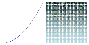
The piece Evaporation was actually produced with a quadratic gradient. Let’s look at a picture first:

That the gradient is quadratic means that the randomness introduced is proportional to $y^2$ for each value of $y.$ In other words, at a level of $y=1/2$ on our square, we subtract a random number between $0$ and

$(1/2)^2=1/4.$

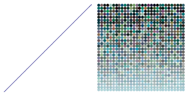
You can visually see this as follows. Look at the gradient of color change from $0$ to $1/2$ for the quadratic gradient. This is approximately the same color change you see in the linear gradient between $0$ and $1/4.$ Why does this happen? Because when you square numbers less than $1,$ they get smaller. So smaller numbers will introduce less randomness in a quadratic gradient than they will in a linear gradient.

We can go the other way, we well. If we use a quadratic gradient (exponent of $2>1$ ), the color changes more gradually at the bottom. But if we use an exponent less than $1$ (such as in taking a root, like a square root or cube root), we get the opposite effect: color changes more rapidly at the bottom. This is because taking a root of a number less than $1$ increases the number. It’s easiest to see this with an example:

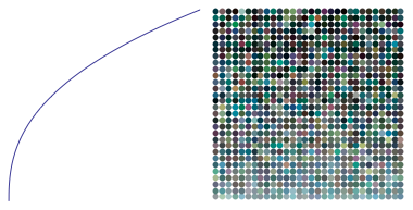
In this case, the exponent used is $0.4,$ so that for a particular $y$ value, a random number between $0$ and $y^{0.4}$ is subtracted from each RGB value. Note how quickly the color changes from the sky blue at the bottom toward very dark colors at the top.

Of course this is just one way to vary colors. But I find it a very interesting application of power and root functions usually learned in precalculus — using computer graphics, we can directly translate an algebraic, functional relationship geometrically into a visual gradient of color. Another example of why it is a good idea to enlarge your mathematical toolbox — you just never know when something will come in handy! If I didn’t really understand how power and root functions worked, I wouldn’t have been able to create this visual effect so easily.

Now it’s your turn! You can visit the Evaporation worksheet to try creating images on your own. If you’ve been trying out the Python worksheets all along, the code should start to look familiar. But a few comments are in order.

First, we just looked at a $1\times 1$ square. It’s actually easier to think in terms of integer variables “width” and “height” (after all, there is no reason our image needs to be square). In this case, we use “j” as the height parameter, since it is more usual to use variables like “i” and “j” for integers. So “j/height” would correspond to $y.$ This would produce a color gradient of light to dark form bottom to top.

To make the gradient go from top to bottom, we use “(height-j)/height” instead (see the Python code). This makes values near the top of the image correspond to $0,$ and values near the bottom of the image correspond to $1.$ I’ll leave it to you to explore all the other details of the Python code.

Please feel free to comment with images you create using the Sage worksheet!

As mentioned in the previous post as well, each parameter you change — each number which appears anywhere in your code — affects the final image. Some choices seem to give more appealing results than others. This is where are meets technology.

As a final word — the work on creating fractals is still ongoing. I’ve learned to make movies now using Processing:

You’ll notice how three copies of one fractal image morph into one of another. You can find more examples on Twitter: @cre8math. Once I feel I’ve had enough experience using Processing, I’ll post about how you can use it yourself. The great thing about Processing is that you can use Python, so all your hard work learning Python will yield even further dividends!

Evaporation I

This and the next post will walk you through how to create digital art similar to Evaporation. I’ll also show you some Python code you can use yourself to experiment.

There are three significant features of Evaporation. First is the randomness of the colors. Second — if you look closely — the sizes of the circles are also different; these are randomly generated as well. The third feature is the gradient of the color — from a pure sky blue at the top, to a fairly randomly colored row of circles at the bottom. We’ll look at the first two features today.

Let’s look at color. In the figure above, the small teal square at the left has RGB values of 0, 0.5, and 0.7, respectively. The larger square at the left consists of 100 smaller squares. The color of each of these squares is generated by adding a random number between 0 and 0.1 to each of the RGB values 0, 0.5, and 0.7 — with a different random number added to each value. In the middle square, a random number between 0 and 0.2 is added, so this creates a wider range of color values. For the right square, the random numbers added are between 0 and 0.3.

But there is no reason that the ranges need to the same for each color. In the images below, the red values have a wider range of randomness then the green, which is “more random” than the blue.

You can see that different ranges of random numbers create different color “textures.” This is where I think computer meets art — as a programmer, when it comes to creating random numbers, you have to specify a range for the randomness of each variable. The choices you make determine how your image looks. How do you make “artistic” choices? There is no easy answer, of course.

Another way to use randomness is by varying the size of the graphic objects. In the left square below, texture is created by randomly changing the radii of the circles.

In the middle square, the circles are all the same size, but random shades of gray. The right square varies both the size of the circles and their color. The final result depends on “how much” randomness is used. You can try it for yourself by altering the Python code linked to below — change the randomness and see what happens!

I think of my laptop as an art laboratory. It is a place to experiment with different ideas — change this parameter, increase randomness, try out different color combinations. Can you imagine creating any of the images in this post by hand? The computer allows us to perform experiments unthinkable to Rembrandt and Van Gogh. We may lose the texture of brush strokes or the dimensionality of paint on canvas, but what we gain by having a programming language at our disposal makes up for this loss. At least in my opinion….

Now let’s look at how we can use Python to create these images. You can experiment with this color and texture worksheet.

There is not much more to say here since a lot is explained in the worksheet. But as you are creating, keep a few things in mind.

1. Use descriptive variable names. This helps a lot when you’re looking a lines of code. Using variables a, b, c, etc., doesn’t help much when you’re looking at a program you wrote a few months ago.

2. Comment liberally! Notes to yourself are easy to use in Python — just start a line (or part of a line) with the “\#” character. You’ll thank yourself later.

3. Save versions often! I won’t bore you with stories of using Mathematica to do some intense computations for creating digital art — and then read the “Mathematica quit unexpectedly” message on my screen — before I saved my work. I’ve encountered this in Python, too — if you use the online version, you’re connecting to an external server, which hopefully will not encounter problems while you’re working….

Also, as you change parameters, you may want to keep track of results you like. If there are a lot of these, sometimes I write the parameters as comments — so I can reproduce them later. Very important: don’t forget to keep track of the random number seed you use! The feel and texture of an image can vary dramatically with the random number seed, so don’t ignore this vital parameter.

One final thought. In creating this type of art, I keep in mind the tension between structure and randomness. You can use the computer to create randomness — but if there’s too much randomness, the image doesn’t seem to hang together. But if there’s too much structure, the image can lose its interesting texture, and appear flat and purely two-dimensional. So the choice of parameters in creating randomness is fairly crucial in determining how the final image will look. And as I’ve said before — this is where technology meets art. It is fairly easy to create a computer-generated image — but not as easy to create computer-generated art. The difference is not exactly easy to describe — and certainly opinions will differ. It is the questions which arise in describing the difference which are intriguing and exciting.

Enough philosophizing. Time to begin the artistic process! Feel free to comment by posting any images you create using the Python code.