March 2017 – Creativity in Mathematics

Mathematics and Digital Art: Update 2

It’s been about a month since my first update, so it’s time for another status report on my second semester teaching Mathematics and Digital Art. It really has been a wonderful semester so far!

Later we’ll look at some student work (like Collette’s iterated function system),

IFSCollette

but first, I’d like to talk about course content.

The main difference from last semester in terms of topics covered was including a unit on L-systems instead of polyhedra. You might recall the reasons for this: first, students didn’t really see a connection between the polyhedra unit and the rest of the course, and second, the little bit of exposure to L-systems (by way of project work) was well-received.

Day007koch1

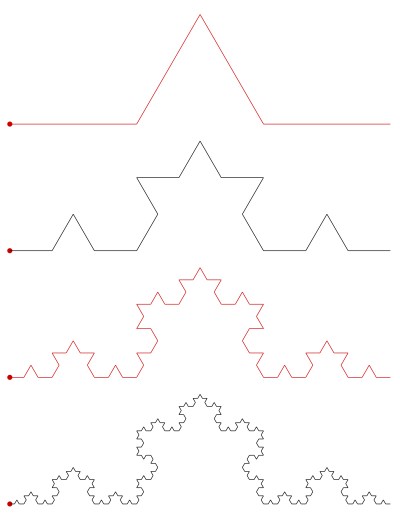
I’ve talked a lot about L-systems on my blog, but as a brief refresher, here is the prototypical L-system, the Koch curve. The scheme is to recursively follow the sequence of turtle graphics instructions

F +60 F +240 F +60 F.

There is also an excellent pdf available online, The Algorithmic Beauty of Plants. This is where I first learned about L-systems. It is a beautifully illustrated book, and I am fortunate enough to own a physical copy which I bought several years ago.

Talking about L-systems is also a great way to introduce Processing, since I have routines for creating L-systems written in Python. Up to this point, we’ve just explored changing parameters in the usual algorithm, but there will a deeper investigation later.

One main focus, however, was just seeing the fractal produced by the algorithm. When working in the Sage environment, the system automatically produced a graphic with axes labeled, enabling you to see what fractal image you created.

In Processing, though, you need to specify your screen space ahead of time. So if your image is drawn off-screen, well, you just won’t see it. You have to do your own scaling and translating, which is sometimes not a trivial undertaking.

I also decided to introduce both finite and infinite geometric series in conjunction with L-systems. This had two main applications.

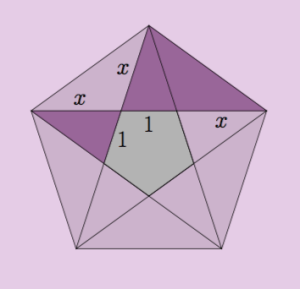
First, we looked at the Sierpinski triangle. Begin with any triangle, and take out the triangle formed by joining the midpoints of the sides. Then repeat recursively, creating the Sierpinski triangle.

Sierp3

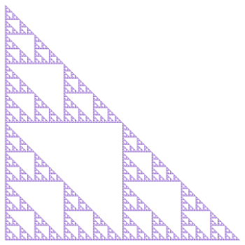
Now assume your original triangle had an area of 1, and calculate the area of all the triangles you removed. Since the process is repeated infinitely, this sum is just an infinite geometric series. Interestingly, the sum of this series is 1, meaning, in some sense, you’ve taken away all the area — but the Sierpinski triangle is still left over! This illustrates an idea not usually encountered by students before: infinite sets of points with no area. Makes for a nice discussion.

Second, we looked at the Koch curve (and similarly defined curves). Using a geometric sequence, you can look at the length of any iteration of the polygonal path drawn by the recursive algorithm. And, as expected, these paths get longer each time, and their lengths tend to infinity as the number of iterations increases. This is another nice way to involve geometric sequences and series.

We’ll be doing more with L-systems in the next few weeks, so I’ll finish this discussion on my next update.

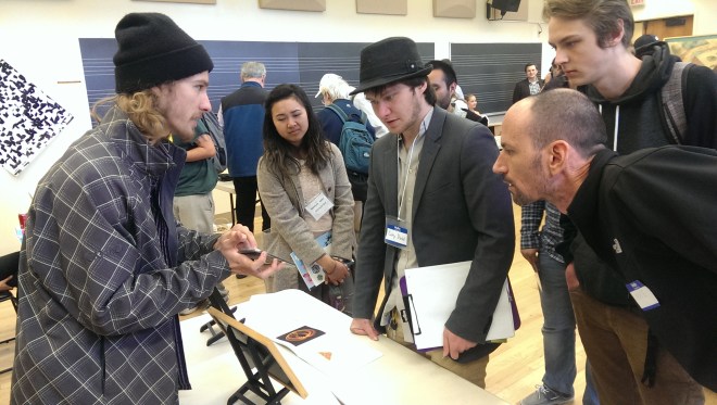
A highlight of the past month was a visit by artist Stacy Speyer.

004 I'llNeverKnow — *I’ll Never Know,* by Stacy Speyer.

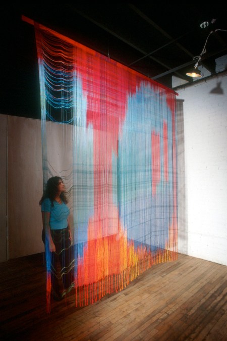
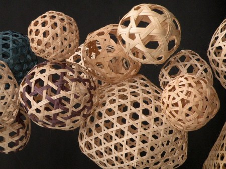
Having worked with weaving and textiles for some time, Stacy has moved on to an investigation of polyhedral forms.

075-WovenGeoInstallVert

Stacy’s talk provided a wonderful insight into integrating mathematics and art in ways we did not study in class. One of the goals of the Bridges papers presentations and the guest speakers is to do precisely this

She writes:

I’m now on a mission to share the fun of making geometric forms with others; I designed Cubes and Things, a 3D coloring book. These easy-to-make paper constructions have patterns that can be colored which emphasize different kinds of symmetric properties of the polyhedra. I bring this fun activity to schools and other groups in the form of Polyhedra Parties. And whenever possible, I still work on making more geometric art and learning more about math.

Visit Stacy’s website to take a look at her book, and view many more examples of her stunning work!

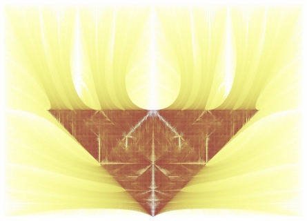
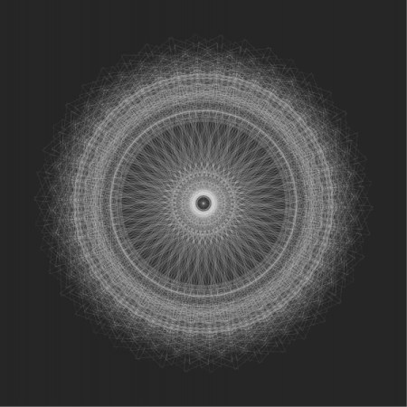
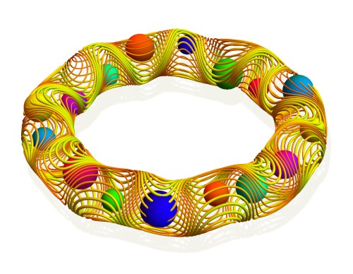
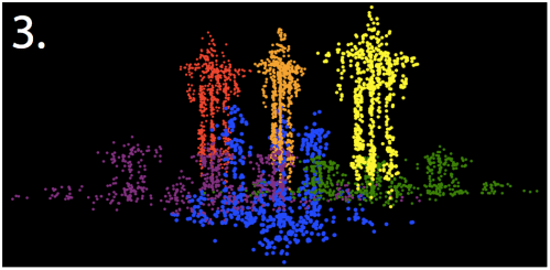
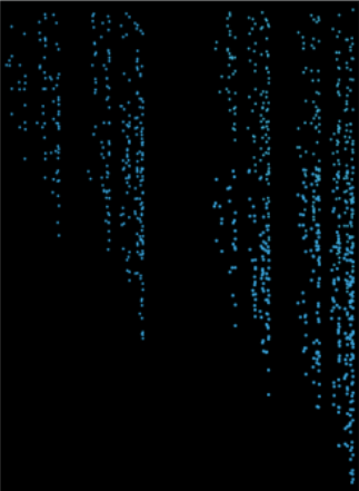
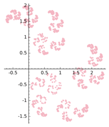
Now we’ll take a look at a few more examples of student artwork. These pieces were submitted for the assignment on iterated function systems. Karla created a piece which reminded her of icicles or twinkling lights.

IFSKarla

Lainey thought her piece looked like a bolt lightning coming out of a wizard’s staff.

IFSLainey

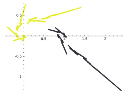
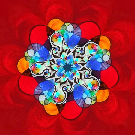
And Peyton’s piece reminder her of flowers.

IFSPeyton

Finally, as I did last semester, I asked students for some mid-semester comments on how the course was going. You can see the complete prompt on Day 19 of the course website. Here are a few of the comments:

I like how it takes a subject that we are all required to take and creates a real, palpable output. Rather than some types of math, where everything is theoretical, it creates a clear chain of events with an even clearer consequence.

[A]fter seeing the kinds of art works there are that involve the kind of math and programming we use, it opened up a new world of artistic possibilities.

What I enjoy most about this course aside from it being small and very interactive in terms of doing labs and having all of our questions answered, is the fact that I would never thought I would be able to create images using programming or math let alone enjoying the satisfaction of the final product.

I was pleased to read these responses, as they suggest the course is fulfilling its intended purpose. But there were also suggestions for improvement — there was a consensus that the math moved a bit too quickly. When we start the discussion on number theory for analyzing the Koch curve next week, I’ll make sure to keep an eye on the pace. I’ll let you know how it goes in my next update in April!

On Coding VIII: LaTeX II

Today, I’ll conclude my remarks about my passion for using LaTeX. As I was writing the last installment of On Coding, I realized that I had more to say than would fit in just one post.

Yet another wonderful thing about LaTeX is how many mathematicians and scientists use it — and therefore write packages for it. You can go to the Comprehensive TeX Archive Network and download packages which make Feynman diagrams for physics, molecular structures for chemistry, musical scores, and even crossword puzzles or chessboards! There are literally thousands of packages available. And like LaTeX, it’s all open source. That is a feature which cannot be overstated. Arguably the world’s best and most comprehensive computer typesetting platform is absolutely free.

The package I use most often is TikZ — it’s a really amazing graphics package written by Till Tantau. You can do absolutely anything in TikZ, really. One extremely important feature is that you can easily put mathematical symbols in any graphic.

tikz1

This is nice because any labels in your diagram will be in the same font as your text. I always find it jarring when I’m reading a mathematics paper or book, and the diagrams are labelled in some other font.

There is so much more to say about TikZ. I plan to talk about it in more detail in a future installment about computer graphics, so I’ll stop here and leave you with one more graphic made with TikZ.

latex2

Another package I use fairly often is the hyperref package. This is especially useful when you’re creating some type of report which relies on information found on the web. For example, when I request funding for a conference, I need to include a copy of the conference announcement. So I create a hyperlink (in blue, though you can customize this) in the document which takes you to the announcement online when you click on it.

These hyperlinks can also be linked to other documents in the cloud, so you can have a “master” document which links to all the documents you need. Now that I’m approaching 100 blog entries, I plan on making an index this way. I’ll create a pdf (using LaTeX, of course) which lists posts by topic with brief descriptions as well as hyperlinks to the relevant blog posts.

On to the next LaTeX feature! I learned about this one from a colleague (thanks, Noah!) when I was writing some notes on Taylor series for calculus. I used it as a text when I taught calculus; the notes are about 100 pages long.

I wanted to share these notes with others, and the style of the notes was such that the exercises weren’t at the end of the sections, but interwoven with the text. Students are supposed to do the exercises as they encounter them.

But for other calculus teachers, it was helpful to include solutions to the exercises. The problem in creating a solutions manual was that if I ever edited the notes, I’d have to also edit the solutions manual in parallel. I knew this was going to happen, since when I gave exams on this material, I added those problems as supplementary exercises to the text.

Enter the ifthen package in LaTeX. I created an exercise environment, so that every time I included an exercise, I had a block which looked like this:

\begin{exercise}

{….the exercise….}

{….the solution….}

\end{exercise}

Think of this as an exercise function with two arguments: the text of the exercise, and the text of the solution.

Then I created a boolean variable called teacheredition. If this variable was true, the exercise function printed the solutions with each exercise. If false, the solutions were omitted. This control structure was made easy by some functions in the ifthen package.

And that’s all there was to it! So every time I created an exercise, I added the solution right after it. Of course the exercises were automatically numbered as well. No separate solutions manual. Everything was all in one place. If you have ever had to deal with this type of issue before, you’ll immediately recognize how unbelievably useful the ability to do this is!

While not really features of LaTeX itself, there are now places in the cloud where you can work on LaTeX documents with others. I’d like to talk about the one Nick and I are currently using, called ShareLaTeX. This is an environment where you can create a project, and then share it with others so they can work on it, too.

So when Nick and I work on a paper together, we do it in ShareLaTeX. It’s extremely convenient. We can edit the paper on our own, but most often, we use ShareLaTeX when we’re working together. Usually, we’re working on different parts of the paper — but when one of us has something we want the other to see, it’s easy to just scroll down (or up) in the document and look at what’s been done.

Also nice is that it’s easy to copy projects — so as we’re about to make a big change (like use different notation, or alter a fundamental definition), our protocol is to make a copy of the current project to work on, and then download the older version of the project (just in case the internet dies).

It’s wonderful to use. And it actually really came in handy when Nick was working on his Bridges paper for last year. His computer hard drive seriously crashed. But since we were working on ShareLaTeX, the draft of his paper was unharmed.

I hope this is enough to convince you that it might be worthwhile to learn a little LaTeX! I seriously don’t know what I’d do without it. And — as it bears repeating — it’s all open source, available to anyone. So, really, why isn’t the whole world using LaTeX? That’s a mystery for another day….

What is…Spherical Geometry?

This week, we’ll look at another type of geometry, namely spherical geometry. Quite simply, this is the geometry of a sphere. Here, a sphere is a set of points equidistant from a given center. In other words, throughout this post, you should imagine only a surface, with nothing inside it — think of the rind of an orange, without any of the slices. I began to describe spherical geometry in my original post, What is a Geometry?, so I’ll briefly summarize the ideas in that post first. It wouldn’t hurt to review it…

From a Euclidean standpoint, there are points on the sphere, but obviously no straight lines. In spherical geometry, we define a Point to be a pair of antipodal points on the sphere, and a Line to be a great circle on the sphere. This results in two nice theorems of spherical geometry: any two distinct Lines determine (intersect in) a single Point, and any two distinct points determine a single Line.

This is a departure from Euclidean geometry, for this means that there are no parallel Lines in spherical geometry, since distinct Lines always intersect. But there is something more going on here.

Consider the statement “Any two distinct Lines determine a single Point.” Now perform the following simple replacement: change the occurrence of “Line” to “Point,” and vice versa. This gives the statement “Any two distinct Points determine a single Line,” and is called the dual of the original statement.

Thus, we have the situation that some statement and its dual are both true. Now if this is true of some set of statements in spherical geometry — that the dual of each statement is true — and we derive a new result from this set of statements, then the following remarkable thing happens. Since the dual of any statement we used is true, then the dual of the new result must also be true! Just replace each statement used to derive the new result with its dual, and you get the dual of the new result as a true statement as well.

This is the principle of duality in mathematics, and is a very important concept. We will encounter it again when we investigate projective geometry.

Triangles and trigonometry are different on the sphere, as well. A spherical triangle is composed of three arcs of great circles, as in the image below.

If this were Earth, you could imagine starting at the North Pole, following 0 degrees of longitude to the Equator (shown in yellow), follow the Equator to 30 degrees east longitude, then follow this line of longitude back to the North Pole.

On the sphere, though, sides of a triangle are actually angles. Sure, you could measure the length of the arcs given the radius of the sphere, but that’s not as useful. Consider the choice of units on the Earth — kilometers or miles? We don’t want important geometrical results to depend on the choice of units. So a side is specified by the angle subtended by the arc at the center of the sphere. This makes sense since the sides are arcs of great circles, and the center of any great circle is the center of the sphere.

The angles between the sides are angles, too! A great circle is just the intersection of a plane passing through the origin and the sphere. So the angle between any two sides is defined to be the angle between the planes which contain them.

Really nothing from Euclidean trigonometry is valid on the sphere. For example, if you look at the triangle above, you can see that the angles between the sides are 30, 90, and 90 degrees. These angles add to 210! In fact, the three angles of a triangle always add up to more than 180 degrees on a sphere. (You may notice that the sides of this triangle are also 30, 90, and 90 degrees, but this is just a coincidence. The sides and angles are usually different.)

If A, B, and C are the angles of a spherical triangle, it turns out that the area of the triangle is proportional to A + B + C – 180. This means that the smaller a triangle is, the closer the angle sum is to 180 degrees.

sphtriangle

There is no Pythagorean Theorem on the sphere, either. In addition, if a, b, and c are the sides opposite angles A, B, and C, respectively, then we have formulas like

$\cos c=\cos a\cos b+\sin a\sin b\cos C$

and

$\cos C=-\cos A\cos B+\sin A\sin B\cos c.$

One interesting consequence of the second of these formulas is this. If you know the angles of a triangle, you can determine the sides. You can’t do this in Euclidean trigonometry, since the triangles may be similar, but of different sizes. In other words, there are no similar triangles on the sphere. Spherical triangles are just congruent, or not. You can’t have two different triangles with the same angles.

For now, we’ve considered our sphere as being embedded in a Euclidean space. The definition of this surface is easy: just choose a point as the center of your sphere, and then find all points which are a given, fixed distance — the radius of the sphere — from that point. Sounds easy enough.

But can you imagine a sphere without thinking of the three-dimensional space around it? Or put another way, imagine you were a tiny ant, on a sphere of radius 1,000,000 km. That’s over 150 times the radius of the Earth! How would you know you were actually on the surface of a sphere? If you were that small and the sphere were that large, it would seem awfully flat to you….

So how could you determine the sphere was curved? This is a question for differential geometry, which among other things, is about the geometry of a surface without any reference to a space it’s embedded in. This is called the surface’s intrinsic geometry.

As an example of looking at the intrinsic geometry of the sphere, consider Lines. Now you can’t say they’re great circles any more, since this relies on thinking of a sphere as being embedded in three-dimensional space; in other words, its extrinsic geometry. You need the concept of a geodesic — in other words, the idea of a “shortest path.”

So if you’re the ant crawling between two points on a sphere, and you wanted to take the shortest path, you would have to follow a great circle arc. So it is possible to define Lines only using properties of the surface itself. But the mathematics to do this is really extremely challenging.

Lots of new ideas here — but we’ve just scratched the surface of a study of spherical geometry. You can see how very different spherical geometry is from both Euclidean and taxicab geometry. Hopefully you’re well on your way to wrapping your head around our original question, What is a Geometry?….

Art Exhibition: Golden Section 2017

Yesterday, artists from the Golden Section of the Mathematical Association of America contributed to yet another art exhibition! Each Spring, members of the MAA from Northern California, Nevada, and Hawaii attend a regional conference — this year, at Santa Clara University.

rectangletriangle — *Woven,* by Nick Mendler.

Last year the event was held at the University of California, Davis, and Shirley Yap from California State University, East Bay organized a highly successful exhibit — what we believe to be the first art exhibition ever to be a part of a sectional MAA meeting. I asked Shirley to say a few words about what motivated her to take on this task.

I exhibited an art piece at the Joint Mathematics Meetings in 2016. It was an interactive piece and I wanted to see how people would experiment with it. So I just hung around the exhibit for a while and not only saw how people played with my piece, but how they observed other pieces. The kind of delight that came from people’s faces convinced me that the art was really drawing them to math in a way that was different from how I had seen before. Perhaps because one is expected to sit in front of art for a long time to contemplate it, people felt relaxed enough to enjoy it. Whatever it was I saw, I knew that I wanted to share the experience with others outside of the JMM.

When we put a call for artists out on our Golden Section website, we didn’t get any responses. So I went through years of JMM art exhibit catalogs and looked up each artist to see if they lived in our section. Then I just started emailing them individually to ask if they were interested in showing their work at a local exhibition.

This year, I offered to help Shirley with organizing the exhibition. Given what was involved in the second year, I have a new appreciation for Shirley’s dedication to spreading the word about mathematical art. Such events do not organize themselves — and we are all grateful Shirley took on this huge task to start a new Golden Section tradition.

redmandalalores — *Red Mandala,* by Frank Farris.

We didn’t have as many artists participate this year — but that’s part of the ebb and flow of yearly events like these. But the quality has high, as was the enthusiasm of the artists. Two of the artists this year were undergraduates — Nick Mendler from the Univiersity of San Francisco, and Juli Odomo from Santa Clara University. I think of them as future organizers of sectional MAA art exhibits….

In the morning, we had the usual opening remarks and a series of excellent speakers. The art exhibit took place in parallel with the Student Poster Sessions, which took place after lunch from 1:00-2:30. This was followed by another series of talks. You can see the full program here.

phil — *Islamic 8-fold Fractal Flower (Median),* by Phil Webster.

I asked the artists to say a few words about their experience about creating or exhibiting mathematical art. Here a few remarks.

Frank Farris (see artwork above):

I love the idea that we’re entering a golden age of mathematical art. New tools become available all the time and a growing community is finding new creative ways to use them. Can’t wait to see what the next years will bring.

I believe the sentiment in Gwen’s quote resonates very strongly with many mathematical artists.

Gwen Fisher:

The thing that keeps bringing me back to bead weaving is mathematics. Of course, I love colors of glass beads and the way they sparkle, but mostly, I keep returning to my seed beads because I keep finding new ways to use and represent mathematical structures with them.

gwenfisher — *Pixel Painting Number VI “Sunnyvale Boogie Woogie”* by Gwen Fisher.

Nick Mendler (see artwork above):

Since my first sectional meeting last Spring, I’ve continued research into the questions that generated my first mathematical artwork over a year ago.
Recognizing that my projects and thoughts are the most rewarding when realized through an aesthetic process has been not only productive, but has been a fascinating source of guidance to new questions. That focusing on more elegant images brings about more elegant mathematics has been only too clear from the sessions I’ve attended so far; I’m looking forward to seeing and learning from more art pieces!

Interested in organizing an art exhibit in your section? Since I helped Shirley with the organizational details this year, I can say a bit about what’s involved in putting together an exhibition.

imag5546 — Intense discussion about mathematical art at the exhibition.

The first step is, clearly, finding artists who want to show their work. It would be easier to get a student worker to do the search Shirley undertook — but don’t forget about the exhibitions at the Bridges conferences! Here is a link to both JMM and Bridges galleries. You can also contact the SIGMAA-ARTS and request that an email blast be sent to members.

koch336_19_107 — *Symmetric Koch Curve I,* by Vince Matsko.

As far as the submission process goes, that’s pretty standard. While it is always nice to accept every submission, sometimes it just isn’t possible. The works should have some real mathematical content, and be of good quality.

Since not all artists necessarily have business cards (especially student artists), I had the idea of making nametags for those who wanted one. You can download this nametag template in LaTeX if you would like, then edit and print onto cardstock. (Note: WordPress would not let me upload a .tex document, so I saved it as an Open Office document.)

It is a good idea to have an assistant or a student helper in the exhibition venue during the conference. Not all artists attended the meeting, and so brought in their work at various times during the day.

Shirley had the wonderful idea of arranging a dinner for contributing artists after the conference. Last year we went to an excellent Thai restaurant, and this year, Frank Farris generously offered to host a pot luck dinner (he provided the lasagna) at his house. These have been very wonderful events, and give artists the opportunity to get to know each other a little better.

A subset of the artists at the celebratory post-exhibition pot-luck. (Photo by Frank Farris.)

Finally, I wanted to mention that I am in the middle of my second time teaching Mathematics and Digital Art at the University of San Francisco. I say this in the event you are interested in offering such a course at your university. I have written extensively about this experience on my blog, and also have all course materials as well as a day-by-day outline available on the Fall 2016 course website. I would be happy to help you get such a course off the ground if you’re interested.

If you would like more information, or want to get in touch with any of the artists whose work is shown above, please make a comment and I’ll get back to you. I hope this is just the beginning of a long tradition of having mathematical art exhibits at sectional MAA meetings!