July 2016 – Creativity in Mathematics

Vienna!

Last week, I attended the Symmetry Festival 2016 in Vienna! I’d like to share some highlights of the week.

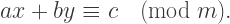
The first was a sculpture based on a hypercube net. One of the most famous illustrations of this geometrical object is Dali’s Crucifixion.

300px-Dali_Crucifixion_hypercube

Without going into too many details, eight cubes may be folded into a four-dimensional cube — called a hypercube or tesseract — just as a net of six squares may be folded into a cube. Because folding a flat net of six squares requires folding into the third dimension, folding a hypercube net requires a fourth spatial dimension.

Analogously, just as the squares are not distorted as they are folded into the third dimension, the cubes are not distorted when folded into the fourth dimension. A little mind-blowing, but true.

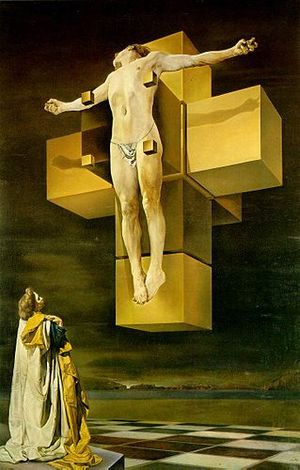
Silas Drewchin created the following sculpture based on the hypercube net.

You’ll notice a few differences: there is an extra cube added, for a total of nine cubes. And there are three additional struts added to support the net being tilted at an angle. Here is what he says about those design elements:

The Hypercross is a metaphor of acceptance….By giving the Hypercross an extra base cube, the mathematical purity of the net tesseract is shattered because a true tesseract only has two base cubes. To disfigure the purity of Christian symbolism embedded in the tesseract, it is tilted to an acute angle as if it is tumbling to the ground. Without this tilted adaptation the sculpture would look dogmatic. The hybrid distortions of the mathematical form and religious form actually add to the message of acceptance.

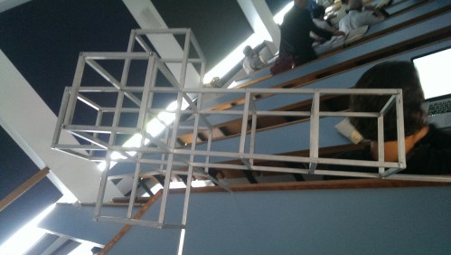
An additional feature of this work relates to the shadows it casts. The photo speaks for itself.

Screenshot 2016-07-24 03.33.42

A fascinating piece! I’m a big fan of the fourth dimension, and always appreciate when it arises in mathematical and artistic contexts.

The second highlight for me was meeting someone who is interested in creating the same type of digital images I do. I had met Paul Gailiunas before at previous conferences, but never knew of his interest. Here is an adaptation of one of his images — you’ll notice a similarity to those I recently posted on Twitter (@cre8math, 2016 July).

ThreeAngles20Jul16

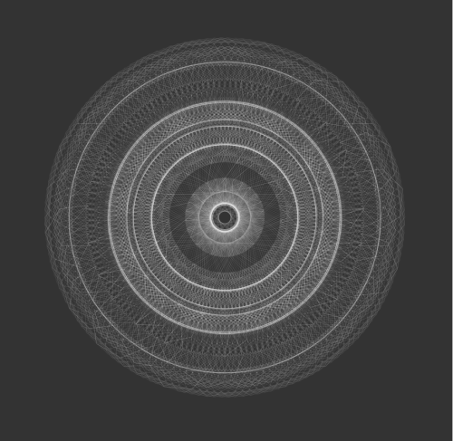
What was facscinating to me was how he created images like these. I first discussed these images on Day007, where I used the same recursive algorithm typically used to create a Koch snowflake:

F +60 F +240 F +60 F.

But Paul used a different recursive algorithm, which I’ll briefly describe — it definitely has a similar flavor, but there are important differences. Define a function R so that R(1) means move forward and make a turn of some specified angle a, and R(2) means move forward and make a turn of some angle b. Then recursively define

R(n) = R(n – 1) R(n – 2).

For example, choosing n = 3 gives the two segments produced by

R(3) = R(2) R(1).

But to obtain R(4), we need to use recursion:

R(4) = R(3) R(2) = R(2) R(1) R(2).

This recursive process may be repeated indefinitely.

This algorithm, like the one used to generate the Koch curve, sometimes closes up and exhibits rotational symmetry. One challenge in this case is that the center of symmetry is not the origin of the coordinate system! A rigorous mathematical proof of which choices of angles a and b generate a closed, symmetric curve is still forthcoming….

A third highlight was the Family Day activities in front of the Karlskirche in the Karlsplatz. At conferences like these (such as the upcoming Bridges conference in Finland), there is a day where mathematics and art activities take place in a public venue, and anyone walking by can sit down and participate.

I sat down at the table demonstrating the Poly-Universe, a system of geometrical forms created by Janos Saxon-Szasz. They were fun to play with, and rather challenging as well!

IMAG2430

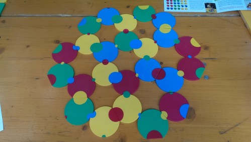
I was happy to have solved the puzzle illustrated here — put together all 24 tiles to make a system of hexagons so that the colors and shapes all match. There are many solutions, but none are easy to find.

What makes these forms interesting is that each tile includes four colors and parts of four differently sized circles. Moreover, they occur in all possible combinations — and since there are 4 sizes of circles, there are 4! = 24 possible configurations.

There are also forms made from triangles and squares, which pose a different challenge. I moved to help a young girl and her mother try to put together a 6 x 4 rectangle from the 24 square pieces, but was not so successful there. At some point you have to move on to see the other exhibits….

A final highlight was the Natural History museum in central Vienna. They had an extensive array of minerals and gems — the largest collection I’ve ever seen. The colors and textures were diverse and beautiful, and of course when looking at crystal structures, there’s a lot of geometry.

Because the rhombic dodecahedron is space-filling, it tends to occur as the basis for crystal structures, as shown here.

IMAG2436

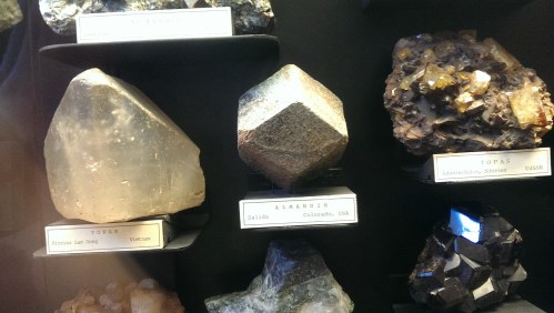
It is always remarkable to me how nature is constrained by geometry — or maybe geometry is derived from nature? Regardless of how you look at it, the interaction of geometry and nature is fascinating.

The week went by pretty quickly, as they usually do when attending conferences like these. Stay tuned for further updates on my European adventure! (I’m also tweeting daily at @cre8math.)

Bridges: Mathematics and Art II

As I mentioned in my first post about Bridges 2016 (see Day038), one of my students, Nick, had artwork and a short paper accepted, and also received a $1000 travel scholarship! This week, I’d like to share his work with you. His paper is called Polygon Spirals. Here is the abstract (all quotes are taken directly from Nick’s paper):

Logarithmic spirals may be classically constructed with a chain of similar triangles that share the same center of similitude. We extend this construction to chains of $n$ -gons with centers on a logarithmic spiral with turning angle $\pi/n,$ and scale factors with interesting properties. Finally, polygon spirals of this kind are used to produce a variety of artistic images.

I first learned of Nick’s interest in this type of spiral when he was in my Calculus II class, where he introduced a similar idea for his Original Problem assignment (see Day013). I encouraged him to continue with this project and submit his work to Bridges 2016. Here is Nick’s motivation in his own words:

The investigation of polygon spirals began by studying curves that arise when regular polygons with an odd number of sides are strung together. When polygons are strung together into a band by gluing them together along their sides, then the choice of what subsequent edge pairs are being used will define a turning angle introduced at each joint. In this paper we focus on bands made with minimal turning angles and with a consistent turning direction. Each odd $n$ -gon defines its own turning angle, $\pi / n.$ Moreover, by introducing a constant scale factor that modifies each subsequent polygon, a large variety of logarithmic spirals can be generated.

My original inspiration came from observing spirals of opposite handedness emerging from adjacent faces of the same polygon. The natural question that arose was which ratio to pick so that the two polygon chains would fall in phase, as in Figure 2. In other words, I needed to find the ratio such that every crossing point of the two logarithmic spirals coincided with the center of a polygon along each band. In this case, the two bands would share a polygon every period. I found this to be achieved when the golden ratio was applied to pentagons, which spurred a determination of the analogous ratio for generalized $n$ -gons that corresponds to the sharing of every $n^{\rm th}$ polygon. The construction hinges on similar triangles whose vertices are the center of a polygon, the center of one of that polygon’s children, and the center of similitude.

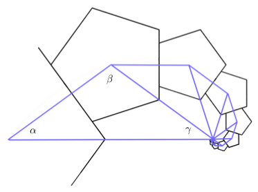
spiral — Figure 3: Logarithmic similar triangles

Referring to Figure3 (illustrated in the case $n=5$ ), $\alpha=\pi/n$ and $\beta=3\pi/n,$ so that $\gamma=\pi/n.$ Now the triangle with angles labelled $\alpha,$ $\beta,$ and $\gamma$ is isosceles because $\alpha = \gamma.$ Moreover, the ratio between the longer and shorter sides is the same for all triangles since the spiral is logarithmic. If the shorter sides are of unit length, half of the base is $\cos (\pi/n),$ making the base, and thus the ratio, equal to $2\cos (\pi/n).$

Once the ratio has been found, spirals can be nested by applying a rotation of $\pi/n.$ Completing this process yields $n$ nested $n$ -gon spirals.

With the ratio found above, it is not hard to show that the equation for one of the logarithmic spirals with this ratio, passing through the centers of the $n$ -gons, has the equation:

$r = (2\cos (\pi/n)) ^{n \theta/{\pi}}.$

With most Bridges papers, there is a mix of mathematics and art. In fact, the first criterion listed on the Bridges website for art submissions is “Math content (this is a mathematically sophisticated audience.)” The second is “Esthetic appeal,” so artistry is important, too. What follows is Nick’s discussion of how he used the mathematical ideas discussed above to create digital art.

Begin with a base polygon, and consider producing spirals from every face at every iteration. Although this would create too dense a pattern, it is possible to produce an interesting subset of this set of polygons using a random algorithm. This algorithm assigns a probability that a spiral is generated from each face of the $n$ -gon, and this probability is randomly altered and then inherited by each child. The colors are also inherited and altered every generation. In Figure 5, the detailed texture is actually built of many small pentagons at a deep iteration. Off to the right can be seen a randomly generated pair of pentagonal arms falling into phase.

Figure 6 is a tiling of pentagons that features nested rings of pentagons with the property that any two adjacent pentagons differ in size by a ratio of the golden ratio. Figure 7 is an overlay of nonagon spirals with ratios between 0 and 1. This image captures the vast breadth of possible spirals based on a given $n$ -gon, and the fascinating way that they interact.

Figure 8 was randomly generated by the same algorithm which produced Figure 5, however with nonagons rather than pentagons. This picture illustrates the infinite detail of a fractal set based on interacting nonagon spirals.

Quite an amazing sequence of images! Nick took a Python programming class his first semester, and so was well-versed in basic coding. As a mathematics major, he had the necessary technical background, and being a double major in art as well helped him with the esthetics.

So yes, it took a lot of work! But the results are well worth it. Nick’s success illustrates what motivated undergraduates can accomplish given the appropriate encouragement and support. Let’s see more undergraduates participate in Bridges 2017!

Mathematics and Digital Art IV

This week will complete the series devoted to a new Mathematics and Digital Art (MDA) course I’ll be teaching for the first time this Fall. During the semester, I’ll be posting regularly about the course progression for those interested in following along.

Continuing from the previous post, Weeks 7 and 8 will be devoted to polyhedra. While not really a topic under “digital art,” so much of the art at Bridges and similar conferences is three-dimensional that I think it’s important that students are familiar with a basic three-dimensional geometric vocabulary.

Moreover, I’ve taught laboratory-based courses on polyhedra since the mid 1990’s, and I’ve also written a textbook for such a course. So there will be no problem coming up with ideas. Basic topics to cover are the Platonic solids (and proofs that there are only five), Euler’s formula, and building models with paper (including unit origami) and Zometools.

There are also over 50 papers in the Bridges archive on polyhedra. One particularly interesting one is by Reza Sarhangi about putting patterns on polyhedra (link here). Looking at this paper will allow an interested student to combine the creation of digital art and the construction of polyhedra.

At the end of Week 7, the proposal for the Final Project will be due. During Week 8, I’ll have one of the days be devoted to a construction project, which will give me time to go around to students individually and comment on their proposals.

This paves the way for the second half of the semester, which is largely focused on Processing and work on Final Projects.

In Weeks 9 and 10, the first two class periods will be devoted to work on Processing. I recently completed a six-part series on making movies with Processing (see Day039–Day044), beginning with a very simple example of morphing a dot from one color to another.

These blog posts were written especially for MDA, so we’ll begin our discussion of Processing by working through those posts. You’ll notice the significant use of IFS, which is why there were such an important emphasis during the first half of the course. But as mentioned in the post on Day044, the students in my linear algebra course got so excited about the IFS movie project, I’m confident we’ll have a similar experience in MDA.

The third class in Weeks 9 and 10 will be devoted to work on the Final Project. Not only does taking the class time to work on these projects emphasize their importance, but I get to monitor students’ progress. Their proposals will include a very rough week-by-week outline of what they want to accomplish, so I’ll use that to help me gauge their progress.

What these work days also allow for is troubleshooting and possibly revising the proposals along the way. This is an important aspect of any project, as it is not always possible to predict one’s progress — especially when writing code is involved! But struggling with writing and debugging code is part of the learning process, so students should learn to be comfortable with the occasional bug or syntax error. And recall that I’ll have my student Nick as an assistant in the classroom, so there will be two of us to help students on these work days.

Week 11 will be another Presentation Week, again largely based on the Bridges archives. However, I’ll give students more latitude to look at other sources of interest if they want. Again, we’re looking for breadth here, so students will present papers on topics not covered in class or the first round of presentations.

I wanted to have a week here to break up the second half of the semester a bit. Students will still include this week in their outline — they will be expected to continue working on their project as well. But I am hoping that they find these Presentation Weeks interesting and informative. Rather like a mini-conference in the context of the usual course.

Weeks 12 and 13 will essentially be like Weeks 9 and 10. Again, given that most students will not have written any code before this course, getting them to make their own movies in Processing will take time. There is always the potential that we’ll get done with the basics early — but there is no shortage of topics to go into if needed. But I do want to make sure all students experience some measure of success with making movies in Processing.

Week 14 will be the Final Project Presentation Week. This is the culminating week of the entire semester, where students showcase what they’ve created during the previous five weeks. Faculty from mathematics, computer science, art, and design will be invited to these presentations as well. I plan to have videos made of the presentations so that I can show some highlights on my blog.

Week 15 is reserved for Special Topics. There are just two days in this last week, which is right before Final Exams. I want to have a low-key, fun week where we still learn some new ideas about mathematics and art after the hard work is already done.

So that’s Mathematics and Digital Art! The planning process has been very exciting, and I’m really looking forward to teaching the course this fall.

Just keep the two “big picture” ideas in mind. First, that students see a real application of mathematics and programming. Second, students have a positive experience of mathematics — in other words, they have fun doing projects involving mathematics and programming.

I can only hope that the course I’ve designed really does give students such a positive experience. It really is necessary to bolster the perception of mathematics and computer science in society, and ideally Mathematics and Digital Art will do just that!

Mathematics and Digital Art III

Now that the overall structure of the course is laid out, I’d like to describe the week-by-week sequence of topics. Keep in mind this may change somewhat when I actually teach the course, but the progression will stay essentially the same.

Week 1 is inspired by the work of Josef Albers (which I discuss on Day002 of this blog). Students will be introduced to the CMYK and RGB color spaces, and will begin by creating pieces like this: Albers2

We’ll use Python code in the Sage environment (a basic script will be provided), and learn about the use of random number generation to create pattern and texture. This may be many students’ first exposure to working with code, so we’ll take it slowly. As with many of the topics we’ll discuss, students will be asked to read the relevant blog post before class. While we’ll still have to review in class, the idea is to free up as much class time as possible for exploration in the computer lab.

Week 2 will revolve around creating pieces like Evaporation,

Day011Evaporation2bWeb

which I discuss on Day011 and Day012. Again, we’ll be in the Sage environment (with a script provided). Here, the ideas to introduce are basic looping constructs in Python, as well as creating a color gradient.

Weeks 3–5 will be all about fractals. This is an ambitious three weeks, so we’ll begin with iterated function systems (IFS), which I discuss extensively on my blog (see Day034, Day035, and Day036 for an introduction).

Two

The important mathematical concept here is affine transformation, which will likely be unfamiliar to most students. Sure, they may understand a matrix as an “array of numbers,” but likely do not see a matrix as a representation of a linear transformation.

But there is such a wealth of fascinating images which can be created using affine transformations in an IFS, I think the effort is worth it. I’ve done something similar with a linear algebra course for computer science majors with some success.

I’ll start with the well-known Sierpinski triangle, and ask students to think about the self-similar nature of this fractal. While the self-similarity may be simple to explain in words, how would you explain it mathematically? This (and similar examples) will be used to motivate the need for affine transformations.

In parallel with this, we’ll look at a Python script for creating an IFS. There is a bit more to this algorithm than the others encountered so far, so we’ll need to look at it carefully, and see where the affine transformations fit in. I’ll create a “dictionary” of affine transformations for the class, so they can see and learn how the entries of a matrix influence the linear/affine transformations.

Having students understand IFS in these three weeks is the highest priority, since they form the basis of our work with Processing later on in the semester. As with any course like this, so much depends on the students who are in the course, and their mathematical background knowledge.

With this being said, it may be that most of these weeks will be devoted to affine transformations and IFS. With whatever time is left over, I’ll be discussing fractal images based on the same algorithm used to produce the Koch curve/snowflake (which I discuss on Day007, Day008, Day009, and Day027).

Day007Starburst

The initial challenge is to get students to understand a recursive algorithm, which is always a challenging new idea, even for computer science majors. Hopefully the geometric nature of the recursion will help in that regard.

If there is time, we’ll take a brief excursion into number theory. Without going into too many details (see the blog posts mentioned above for more), choosing angles which allow the algorithm to close up and draw a centrally symmetric figure depends on solving a linear diophantine equation like

$ax+by\equiv c\quad ({\rm mod}\ m).$

It turns out that the relevant equation may be solved explicitly, yielding whole families of values which produce intricate images. Here is one I just created last week for a presentation on this topic I’ll be giving at the Symmetry Festival 2016 in Vienna this July:

Koch_336_210_218

There is quite a bit of number theory which goes into setting up and solving this equation, but all at the elementary level. We’ll just go as far as we have time to.

Week 6 will be the first in a series of three Presentation Weeks. This week will be devoted to having students select and present a paper or two from the Bridges archive. This archive contains over 1000 papers given at the Bridges conferences since 1998, and is searchable.

The idea is to expose students to the breadth of the relationship between mathematics and art. Because of the need to explain both the mathematics and programming behind the images we’ll create in class, there necessarily will be some sacrifice in the breadth of the course content. Hopefully these brief presentations will remedy this to some extent.

With three 65-minute class periods and 13 students, it shouldn’t be difficult to allow everyone a 10-minute presentation during this week. It is not expected that a student will understand every detail of a particular paper, but at least communicate the main points.

Presentations will be both peer-evaluated and evaluated by me. As these are first-year students, it is understood that they may not have given many presentations of this type before. It is expected that they will improve as the semester progresses.

I realize that some of these ideas are repeated from last week’s post, but I did want to make these two posts covering the week-by-week sequence of topics self-contained. I also wanted to give enough detail so that anyone considering offering a similar course has a clear idea of what I have in mind. Next week, we’ll finish the outline, so stay tuned!