Koch curve – Creativity in Mathematics

Recursively Generated Spirals

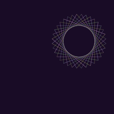
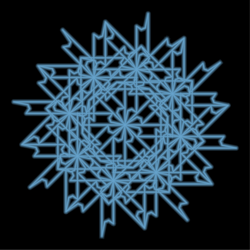
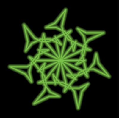
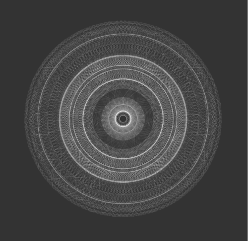
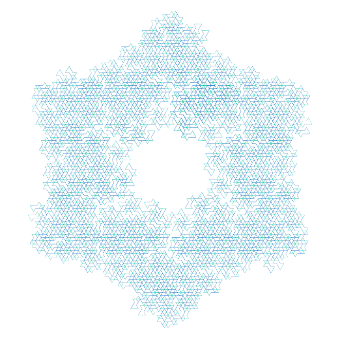
A few weeks, ago I dug out a problem which had puzzled me for over three years. I finally decided that now it was time to really dig in — and to my surprise and delight, not only did I solve the problem, but I’ve already got a draft of a paper written! The figure below is from that paper.

Spiral

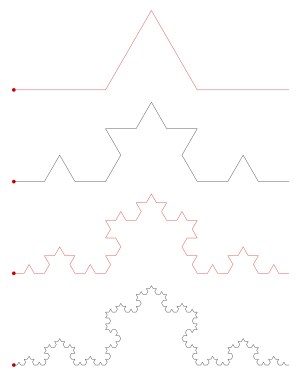
The problem is yet another variation on the recursion which produces the Koch snowflake. I discussed the Koch snowflake in one my first posts, so visit my Day007 post on this fascinating fractal for a refresher.

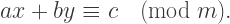
So what is the variation here? Consider the general recursive scheme

${\sf F}\ +\alpha_1\ \ {\sf F}\ +\alpha_2\ \ {\sf F}\ +\alpha_3\ \ {\sf F},$

where ${\sf F}$ represents a forward move and the $\alpha_i$ indicate counterclockwise turns, which would be common instructions in a turtle graphics setting.

The Koch curve is generated by choosing

$\alpha_1=60,\quad \alpha_2=240,\quad \alpha_3=60.$

Previously I’ve studied cases where $\alpha_1=\alpha_3$ and the resulting image possesses central symmetry, unlike the Koch curve (see my Day008 post for examples). But this is my first venture into exploring instances where $\alpha_1\ne\alpha_3.$ Things work a bit differently here….

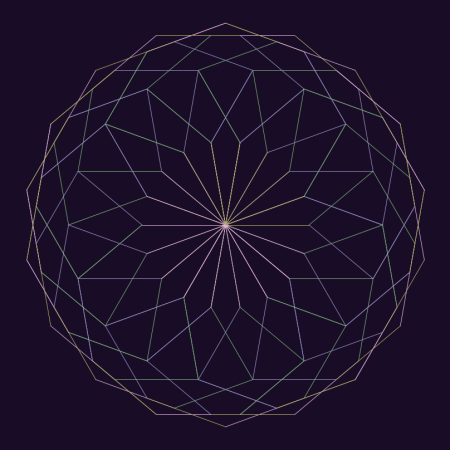
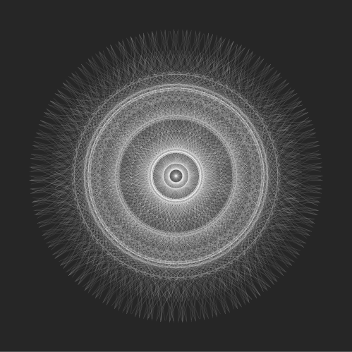
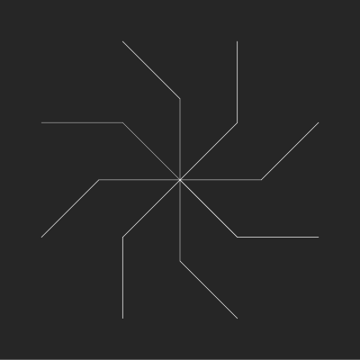
So let’s investigate the example illustrated above in more detail. The recursive scheme which generates this spiral is given by

$\alpha_1=30,\quad \alpha_2=180,\quad \alpha_3=330.$

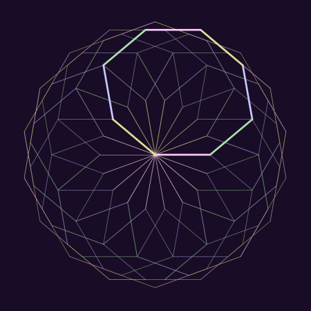
How does this scheme draw a spiral arm? Let’s look at the figure below.

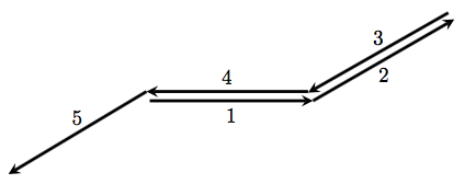
We begin at the origin, and then draw a segment at $0^\circ,$ labeled “1” in the figure. Next, we turn counterclockwise $30^\circ$ (since $\alpha_1=30$ ) and draw the segment labeled “2”.

The next turn is $180^\circ,$ so we turn completely around and begin retracing the arm in the opposite direction. Then turn counterclockwise $330^\circ$ and move forward. Note that since $330=360-30,$ this has the effect of taking us right back to the origin.

What next? It is at this point that we invoke a recursive call — and so the next angle tells us what direction the next arm will be drawn in. Of course, like before, the three angles after that will continue drawing the arm and then bring us back to the origin, awaiting the next recursive call.

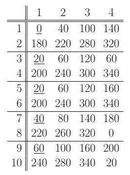
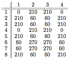
This behavior can be illustrated in the following chart.

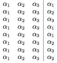
Here, the angles turned are listed in rows of four, one after another. The first three angles in each row are the same, and their job is to complete the arm once a direction is chosen. But the direction chosen is determined by the fourth column (separated by the divider), whose behavior is not periodic and highly recursive.

So where do we go from here? The next chart we’ll look it is a chart of the directions the arms are drawn in.

Sigma4k

We read this chart in rows as follows: the first arm is drawn at an angle of $0^\circ,$ directly to the right. The second arm is drawn at an angle of $210^\circ,$ as can be seen in the figure above.

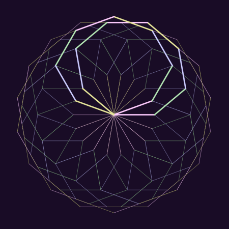
But the third arm exactly retraces the second arm drawn, since it is pointed in the direction of $210^\circ$ as well. The fourth arm drawn — at an angle of $0^\circ$ — exactly retraces the first arm drawn.

So you can see what’s going on. One important consequence of the recursive algorithm is that the arms keep being retraced over and over again.

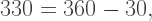
When will the complete spiral be drawn? Well, we need to see every multiple of $30^\circ$ in the chart above. Of course eight rows isn’t enough. But what is really surprising is that it takes over 1,000,000 rows before every multiple of 30 is encountered!

How would you show this? We can’t go into all the details here. The important observation is that if you read across the chart one row at a time, you get the same sequence of angles by reading down the first column of the chart.

But it isn’t enough to just observe this — it has to be proved. This is where some elementary number theory comes in. No more than what might be seen in an undergraduate number theory course, but beyond the scope of this post.

Slight step up on my soapbox — while I usually deplore the definition of mathematics as the “science of finding patterns” (as this only scratches the surface), in this case, finding patterns is critically important. With some trial and error, you hit upon making charts in rows of four, and then putting the directions the arms are drawn in rows of four, and then stare at the numbers until you notice patterns in the charts. The trick is knowing what to prove — once stated properly, the results almost prove themselves.

You’ll have to wait for the paper to come out for all the details. But here is a brief summary. Suppose you divide the circle into n parts, where n is even. Then devise a recursive scheme using the turning angles

$\alpha_1=\dfrac{360}n,\quad\alpha_2=180,\quad\alpha_3=360-\dfrac{360}n.$

Now define

$\sigma(k)=\dfrac13\left(4^{k-1}+2\right),\qquad k\ge1.$

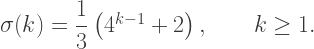
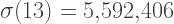
When n is divisible by 4, the spiral has n arms, and you need to draw exactly $\sigma(n+1)$ segments to render the entire spiral. In our case, with 12 arms, it takes $\sigma(13)=5,\!592,\!406$ segments to render the spiral.

But when n is even but not divisible by four, the spiral only has n/2 arms, and it takes $\sigma(n/2+1)$ segments to draw a complete image of the spiral.

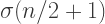
Absolutely amazing, in my opinion. I formulated these conjectures over three years ago, but got stuck. A few weeks ago I had the house to myself for a while, and I just sat down and said to myself, “Look, you’ve already written one paper on these recursions. You can do this.”

And within two days, I worked out the patterns. Then the proofs, and within a week, a draft of the paper.

I am always humbled by such a seemingly innocuous problem — generating a simple spiral . But there are so many levels to this problem, and so much interesting mathematics to be discovered. I’ll continue exploring recursively drawn images, and share the amazing results with you when I find them!

Imagifractalous! 2: p-adic sequences

In Imagifractalous! 1, I talked about varying parameters in the usual algorithm for creating the Koch curve to produce a variety of images, and casually mentioned p-adic valuations. What happened was about a year after I began exploring these interesting images, I did a Google search (as one periodically does when researching new and exciting topics), and stumbled upon the paper Arithmetic Self-Similarity of Infinite Sequences.

It was there that I recognized the sequence of 0’s and 1’s I’d been using all along, and this sequence was called a 2-adic valuation (mod 2).

Here’s the definition: the p-adic valuation is the sequence such that the nth term in the sequence is the highest power of p which divides n. So the 2-adic valuation begins

0, 1, 0, 2, 0, 1, 0, 3, 0, 1, 0, 2, 0, 1, 0, 4, ….

Of course all terms with odd n are 0, and for the even n, you just look at the highest power of 2 dividing that even number. And you can take this sequence (mod 2), or mod anything you like.

I naturally did what any right-thinking mathematician would do — looked up p-adic sequences in the The On-Line Encyclopedia of Integer Sequences. Now it’s not that p-adic valuations are all that obscure, it’s just I had never encountered them before.

Of course there it was: A096268. And if you read through the comments, you’ll see one which states that this sequence can be used to determine the angle you need to turn to create the Koch snowflake.

I wasn’t particularly discouraged — this sort of thing happens all the time when exploring new mathematical ideas. You just get used to it. But something unexpected happened.

I starting experimenting with other p-adic valuations mod 2 (since I had two choices of angles), and found similar interesting behavior. Not only that, p didn’t have to be prime — any integer would do.

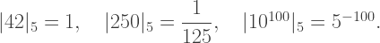
But most papers about p-adic valuations assumed p was prime. Why is that? If $\nu_p$ is a p-adic valuation and p is prime, it’s not hard to show that

$\nu_p(mn)=\nu_p(m)+\nu_p(n),$

an often-used property in developing a theory of p-adic valuations. But it only takes a moment to see that

$\nu_6(4)=0,\quad \nu_6(9)=0,\quad \nu_6(4\cdot9)\ne\nu_6(4)+\nu_6(9).$

Bad news for the p-adic theorists, but the fractal images couldn’t seem to care whether p was prime or not….

Beginning segment of a curve based on a 12-adic valuation.

So I didn’t plunge into researching p-adic valuations, since I needed a treatment which included p composite, which didn’t seem to be out there.

But here’s the neat part. Most of the work I’d done to prove something already known — that a 2-adic valuation (mod 2) could be used to produce a Koch curve — could be used to study generic p. So I was able to make fairly good progress in a relatively short amount of time, since I’d already thought about it a lot before. I suspect it would have taken me quite a bit longer if I’d just casually read about the 2-adic result rather than prove it myself.

The progress made was similar to that of the 2-adic case — number of segments in each arm in the symmetric case, how many solutions given a particular order of symmetry, and so forth.

Now my fractal brain was truly revved up! I enjoyed creating images using various p-adic valuations — the variety seemed another dimension of endless. So I started brainstorming about ways to even further diversify my repertoire of fractal images.

The first two weeks of November were particularly fruitful. Two ideas seemed to coalesce. The first revolved around an old unexplored question: what happened when you didn’t only change the angles in the algorithm to produce the Koch snowflake, but you also changed the lengths?

Of course this seemed to make the parameter space impossibly large, but I was in an adventurous mood, and the only thing at stake was a few moments with Mathematica generating uninteresting images.

Image based on a 3-adic valuation with different edge lengths.

But what I found was that if an image closed up with a particular symmetry, then as long as the sequence of edge lengths was appropriately periodic, the image with different edge lengths also closed up with the same order of symmetry!

This was truly mind-boggling at first. But after looking at lots of images and diving into the algorithm, it’s not all that improbable. You can observe that in the image above, segments of the same length occur in six different orientations which are 60 degrees apart, and so will ultimately “cancel out” in any final vector sum and take you right back to the origin.

Now I don’t have the precise characterization of “appropriately periodic” as yet, but I know it’s out there. Just a matter of time.

The second big idea at the beginning of November involved skimming through the paper on arithmetic self-similarity mentioned above. Some results discussed adding one sequence to another, and so I wondered: what if you added two p-adic sequences before taking their sum (mod 2)?

2016-11-22-8+64adic.png — Imaged based on adding 8-adic and 64-adic valuations with different edge lengths.

Well, preliminary results were promising only when the p-adic valuations involved were of the same power of some p, like in the image above (which also involves different edge lengths).

These ideas are only in a very preliminary stage — it’s the perennial problem of, well, waiting….. It may look liking adding 2-adic and 3-adic valuations doesn’t get you anywhere, but maybe that’s just because you need so many more iterations to see what’s actually happening. So there’s lots more to explore here.

Beginning segment of an image based on a 42-adic valuation.

So as the parameter space gets larger — mutliple different lengths, adding several different p-adic valuations — the variety becomes infinitely diverse, and the analysis becomes that much more involved.

But that makes it all the more intriguing. And it will be all the more rewarding when I finally figure everything out….

Imagifractalous! 1: How it all began.

September 2, 2015 — that was the day Thomas sent an email to the faculty in the math department asking if anyone was willing to help him learn something about fractals. And that was when it all began.

Now I’ve told this story in various forms over the past year or so on my blog, but I want to begin a thread along a different direction. I’d like to give a brief chronological history of my work with fractals, with an eye toward the fellow mathematician interested in really understanding what is going on.

I’ll be formal enough to state fairly precisely the mathematical nature of what I’m observing, so as to give the curious reader an idea of the nature of the mathematics involved. But I’ll skip the proofs, so that the discussion doesn’t get bogged down in details. And of course provide lots of pictures….

You might want to go back to read my post of Day007 — there is a more detailed discussion there. But the gist of the post is the question posed by Thomas at one of our early meetings: what happens when you change the angles in the algorithm which produces the Koch curve?

What sometimes happens is that the curve actually closes up and exhibits rotational symmetry. As an example, when the recursive routine

F +40 F +60 F +40 F

is implemented, the following sequence of segments is drawn.

Now this doesn’t look recursive at all, but rather iterative. And you certainly will have noticed something curious — some sequences of eight segments, which I call arms, are traversed twice.

All of this behavior can be precisely described — all that’s involved is some fairly elementary number theory. The crux of the analysis revolves around the following way of describing the algorithm: after drawing the nth segment, turn +40 degrees if the highest power of 2 dividing n is even, and turn +60 degrees if it’s odd. Then move forward.

I would learn later about p-adic valuations (this is just a 2-adic valuation), but that’s jumping a little ahead in the story. I’ll just continue on with what I observed.

What is also true is that the kth arm (in this case, the kth sequence of eight segments) is retraced precisely when the highest power of power of 2 dividing k is odd. This implies the following curious fact: the curve in the video is traced over and over again as the recursion deepens, but never periodically. This is because the 2-adic valuation of the positive integers isn’t periodic.

So I’ve written up some results and submitted them to a math journal. What I essentially do is find large families of angle pairs (like +40 and +60) which close up, and I can describe in detail how the curves are drawn, what the symmetry is, etc. I can use this information to create fractal images with a desired symmetry, and I discuss several examples on a page of my mathematical art website.

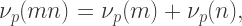
As one example, for my talks in Europe this past summer, I wanted to create images with 64 segments in each arm and 42-fold symmetry. I also chose to divide the circle in 336 parts — subdivision into degrees is arbitrary. Or another way of looking at it is that I want my angles to be rational multiples of $\pi,$ and I’m specifying the denominator of that fraction.

Why 336? First, I needed to make sure 42 divided evenly into 336, since each arm is then 8/336 away from the previous one (although they are not necessarily drawn that way). And second, I wanted there to be enough angle pairs so I’d have some choices. I knew there would be 96 distinct images from the work I’d already done, so it seemed a reasonable choice. Below is one of my favorites. The angles used here are 160 and 168 of the 336 parts the circle is divided into.

koch_336_6_160_168

Now my drawing routine has the origin at the center of the squares in the previous two images, so that the rotational symmetry is with respect to the origin. If you think about it for a moment, you’ll realize that if both angles are the same rational multiple of $\pi,$ you’ll get an image like the following, where one of the vertices of the figure is at the origin, but the center of symmetry is not at the origin.

$fractal_40_60_4$

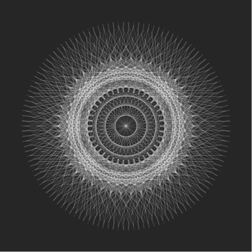
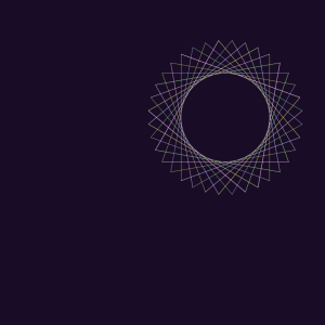
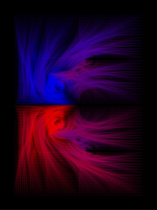
Of course it could be (and usually is!) the case that the curve does not close — for example, if one angle is a rational multiple of $\pi,$ and the other is an irrational multiple of $\pi.$ Even when they do close, some appealing results are obtained by cropping the images.

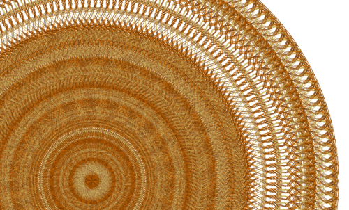
koch-60-254web

So where does this bring me? I’d like a Theorem like this: For the recursive Koch algorithm described by

F $\alpha_0$ F $\alpha_1$ F $\alpha_0$ F,

the curve closes up precisely when (insert condition on $\alpha_0$ and $\alpha_1$ ), and has the following symmetry (insert description of the symmetry here).

I’m fairly confident I can handle the cases where the center of symmetry is at the origin, but how to address the case when the center of symmetry is not the origin is still baffling. The only cases I’ve found so far are when $\alpha_0=\alpha_1,$ but that does not preclude the possibility of there being others, of course.

At this point, I was really enjoying creating digital artwork with these Koch-like images, and was also busy working on understanding the underlying mathematics. I was also happy that I could specify certain aspects of the images (like the number of segments in each arm and the symmetry) and find parameters which produced images with these features. By stark contrast, when I began this process, I would just randomly choose angles and hope for the best! I’d consider myself lucky to stumble on something nice….

So it took about a year to move from blindly wandering around in a two-dimensional parameter space (the two angles to be specified) to being able to precisely engineer certain features of fractal images. The coveted “if-and-only-if” Theorem which says it all is still yet to be formulated, but significant progress toward that end has been made.

But then my fractal world explodes by moving from 2-adic to p-adic. That for next time….

p-adic Numbers II: When Big is Small

Today we’ll finish our brief introduction to p-adic numbers. It’s been a few weeks, so it couldn’t hurt to skim over the first post to refresh your memory.

6adicglow2

After we finish our discussion of …..4444444, we’ll look at how to use ideas related to p-adic numbers to create fractal images like the one above.

Recall that our goal was to show that in the field of p-adic numbers, we had

$.....444444444 = -1.$

I should point out that the term field in mathematics has a very specific meaning, but we won’t be going into any more details about fields here.

In preparing to show this, we defined the 5-size of a number to be

$|n|_5=\dfrac1{5^q},$

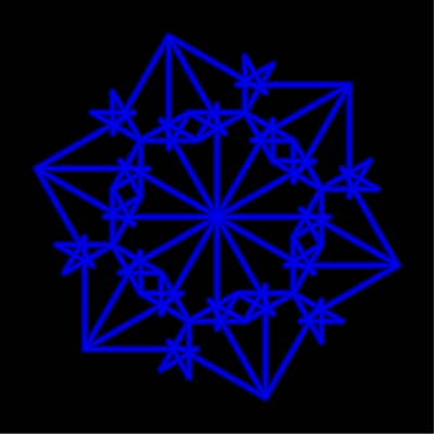
where $5^q$ is the largest power of 5 which is a factor of n. Although unconventional, this distance function satisfies all the necessary properties.

Here is where things get really interesting! While thinking in terms of ordinary distance, it seems that the terms in the sequence of numbers

$4, 44, 444, 4444, 44,\!444, \ldots$

keep getting further and further apart. But in terms of the 5-size, they actually get closer together.

Let’s see why. The 5-distance between 4 and 44 is

$|44-4|_5=|40|_5=\dfrac15,$

since 5 is the largest power of 5 going into 40. Recall that we’re working in base 5, so that in fact

$40_5=20_{10}.$

So the highest power of 5 going into a number, written in base 5, is the number of 0’s at the end of that number.

Next, the distance between 44 and 444 is

$|444-44|_5=|400|_5=\dfrac1{25},$

since $5^2$ is the largest power of 5 dividing 400.

Can you see where we’re going with this? If you subtract a number with $n$ fours from a number with $n+1$ fours, you get $4\cdot5^n,$ and so the 5-distance between them is $|4\cdot5^n|_5=1/{5^n}.$ Therefore, as you keep adding fours, the numbers actually get closer and closer together when you consider the 5-size of their respective differences.

In mathematical terms, we say the sequence

$4, 44, 444, 4444, 44,\!444, \ldots$

converges with respect to the 5-distance, much as we say that $0.999999999.....$ converges with respect to the usual distance on real numbers.

What does this sequence converge to? Suppose that

$.....444444444 = L.$

Let’s try to find L. This is where addition modulo 5 comes in! Consider the following addition problem:

$\begin{tabular}{r}.....444444444\\1\\ \hline .....000000000\end{tabular}.$

We’ll take a moment to interpret this sum. On the very right (the units place), we add 1 + 4. But that’s 5, and there is no digit “5” in base 5 — rather, we write “10.” This means write down the 0, and carry the 1. But then in the second column from the left (the 5’s place), we have 1+ 4 = 10, and so we write down the 0 and carry the 1.

As you can see, this process never ends, and the result is an infinite string of 0’s, which is 0. This shows that

$.....444444444 + 1 = 0,$

or, in other words,

$.....444444444 = -1!$

And here’s the really mind-blowing part. Consider the geometric series

$4+40+400+4000+40,\!000+\cdots,$

in base 5. The first term is 4, and the common ratio is 5. So the sum is

$\dfrac{a}{1-r}=\dfrac4{1-5}=-1.$

Yes, the geometric series formula works when r is 5! The reason is that when you keep multiplying numbers by 5 in the field of p-adic numbers, you’re really bringing them closer together. Sounds impossible — but this can all be rigorously proved in the world of p-adic numbers.

Though we’ve only taken a small peek at the world of p-adic numbers, I’d like to take a few moments to say why they are significant when it comes to creating fractal images. After all, that was the reason I found out about p-adic numbers in the first place!

On Day008, I discussed a way to determine which way you need to turn at any point during the construction of the Koch curve. Here are the first few iterations of the Koch curve algorithm, in case you’ve forgotten.

Day007koch1

In that post, I said I “discovered” that at step n, all you needed to do was look at the highest power of 2 going into n, and turn one way if that power was even, and another way if that power was odd.

But if you think about it for a moment, this is just what we did to calculate 5-size — found the highest power of one number which divides another number. And if we just look at those exponents, we get what’s called a 5-adic valuation. The first several terms look like this:

$0,0,0,0,1,0,0,0,0,1,0,0,0,0,1,0,0,0,0,1,0,0,0,0,2,0,0,0,0,1,0,....$

Any number not divisible by 5 has a valuation of 0, multiples of 5 have a valuation of at least 1, although for 25, you get 2. And so on.

Actually, just a few weeks ago, I read in a paper I found online that the Koch curve can be generated by a 2-adic valuation. As often happens in experimenting with mathematical ideas, you often re-discover ideas someone else already knew about.

I didn’t really care, though. Doing mathematics is as much about the process as the result, and I really had fun “discovering” this, and writing my own proof showing how it generated the Koch curve.

So this got me thinking. If you can generate fractal images with a 2-adic valuation, why not try a p-adic valuation for some value of p different from 2?

And to my amazement, it works in very much the same way! But in order to generate a curve using two angles, you have to take the p-adic valuation, and then take it mod 2. This generates a sequence of 0’s and 1’s, and that’s all you need.

I also found out that my work reproving an old result actually helped a lot — since I was able to prove a similar result for curves generated by a p-adic valuation in almost exactly the same way. And my previous work already had me thinking about the relevant features of these new curves. So when you discover some cool mathematical fact that someone else already knew, well, don’t despair. Just entertain the thought that great minds think alike….

I’ve been experimenting a lot with p-adic valuations recently — this image is based on a 3-adic valuation. I’ll only say that this opens up an entire new world of fractal image possibilities. Check out my Twitter @cre8math for more cool examples!

p-adic Numbers I: When Big is Small

I can’t resist sharing something I just learned about this week. p-adic numbers! I discovered them while exploring angle sequences in creating Koch-like curves, and was immediately fascinated by them. For example, we’ll see that in the field of 5-adic numbers,

$.....444444444 = -1.$

That’s right — the integer with infinitely many 4’s strung together is actually equal to $-1$ ! This seems impossible at first glance, but is actually closely related to

$0.999999999..... = 1$

using decimal numbers.

The subject of p-adic numbers is a broad area in number theory, and we’ll only get a chance to take a small glimpse into it. The simplest examples to look at are related to geometric series. We’ll briefly review them to refresh your memory.

Recall that

$a+ar+ar^2+ar^3+\cdots ar^n+\cdots=\dfrac a{1-r}$

when either $a=0$ or $|r|<1.$

When $r=1,$ for example, the series

$2+2+2+2+2+\cdots$

diverges. To see this, we need to take the sequence of partial sums

$2, 2+2, 2+2+2, 2+2+2+2,\ldots = 2, 4, 6, 8, \ldots,$

which keeps getting larger and larger. By contrast, the series

$1+\dfrac12+\dfrac14+\dfrac18+\cdots\dfrac1{2^n}\cdots$

converges because the sequence of partial sums

$1,1+\dfrac12,1+\dfrac12+\dfrac14,1+\dfrac12+\dfrac14+\dfrac18,\ldots=1,\dfrac32,\dfrac74,\dfrac{15}8,\ldots$

keeps getting closer and closer to 2. Of course we can verify the sum with the formula

$\dfrac{a}{1-r}=\dfrac 1{1-1/2}=2.$

The key idea behind discussing convergence is creating a precise mathematical definition of “getting closer and closer to.” This is done using limits (we will not need to go into details here) and the distance function on the real numbers:

$d(x,y)=|y-x|.$

Intuitively, the absolute value of the difference between two numbers is an indication of how close they are.

For a sequence like

$4, 44, 444, 4444, 44,\!444, \ldots,$

which are the partial sums of the geometric series

$4+40+400+4000+40,\!000+\cdots,$

it seems that the terms keep getting further and further apart:

$d(444,4444)=4000,\quad d(4444,44,\!444)=40,\!000,....$

In the field of p-adic numbers, closeness is measured a different way. This might sound strange at first, but let’s consider closeness in plane geometry for a moment.

We are all familiar with the usual distance function in Euclidean geometry:

$d((x_1,y_1),(x_2,y_2))=\sqrt{(x_2-x_1)^2+(y_2-y_1)^2}.$

But maybe you weren’t aware that there are other ways to define distance in the plane — in fact, infinitely many ways — which give rise to non-Euclidean geometries. One of the simplest is

$d_T((x_1,y_1),(x_2,y_2))=|x_2-x_1|+|y_2-y_1|.$

This is often called the taxicab distance, since it describes how far it is from one point to another if you took a taxi on a rectangular grid of streets.

For example, consider going from (0,0) to (3,2) — we’ll use blocks as units — if you could only walk north, south, east, or west. The shortest path might be to go east three blocks, and then north two blocks. Or perhaps north one block, east three blocks, and then north one block again. But the shortest path will always require that you walk five blocks, since you aren’t allowed to walk along a diagonal path. (Note that the shortest path is not always unique in taxicab geometry!)

This is a perfectly legitimate geometry, with its own set of properties. For example, the “unit circle” described by the equation

$d_T((x,y),(0,0))=|x|+|y|=1$

is in fact not a circle at all, but a square with vertices at a distance of 1 along the axes!

taxicab

But not any function for distance will work — for example, you’ve got to make sure the triangle inequality is still valid (and it is in taxicab geometry). So while some properties still need to hold, most other properties won’t.

What does this have to do with p-adic numbers? We’re going to look at the positive integers for now, but define close in a very different way. So we can look at some specific examples, let’s take $p=5.$

Here’s the big leap: we say a positive integer is 5-small if there are many factors of 5 in its prime factorization. More specifically, if q is the largest power of 5 which is a factor of n, then the we say that its 5-“size” is

$|n|_5=\dfrac1{5^q}.$

Here are a few more examples, which you should be able to work out for yourself.

$|42|_5=1,\quad |250|_5=\dfrac1{125},\quad |10^{100}|_5=5^{-100}.$

But not everything big is small! For example,

$|10^{100}+1|_5=1,$

since there are no factors of 5 present (which is true for any number ending in a 1).

This may seem odd at first, but when you read more about it, it’s actually amazing. I’ll have to admit that to understand a lot of the amazingness, you’d have to go to grad school in mathematics…. But we’ll get to look at a litte bit of it here.

Before we do, though, there’s another role that 5 plays. We’ve got to write 5-adic numbers in base 5. There’s not room to go into all the details here, but we’ll give a brief review.

Recall that in base 10, we have

$5432_{10}=2+3\times10+4\times10^2+5\times10^3.$

We can only use the digits 0–9.

Now in base 5, we can only use the digits 0–4, and we interpret the digits as follows:

$4302_5=2+0\times5+3\times5^2+4\times5^3=577_{10}.$

We add the same way as we do in base 10, except we carry when we add to more than 5 (and not 10). Thus,

$4_5+3_5=12_5,\quad 34_5+12_5=101_5.$

Subtraction, multiplication, and division are handled similarly.

You won’t need to be an expert in base-5 arithmetic in order to understand how this applies to the equation

$.....444444444 = -1.$

But that will have to wait for the next post on p-adic numbers! We’ll see why this is true, and maybe even talk a little bit about rational p-adic numbers, too….

Koch Curves and Canopies

Time for another “math in the moment” post! There have been a few interesting developments just this past week, so I thought I’d share them with you.

The first revolves around the Koch curve. I’ve talked a lot about the algorithm used to generate the Koch curve when the angles are changed — but this is the first time I’ve experimented with three different angles. For example, the recursive procedure

F +45 F +180 F +315 F

generates the following spiral:

spiral8

Looks simple, right? Just 16 line segments. But here’s the unexpected part — it takes 21,846 iterations to make! That’s right — the horizontal segment in the upper left is the 21,846th segment to be drawn.

Why might this be? Partly because of the fact that one angle is 180, and also the fact that 45 + 415 = 360. In other words, you are often just turning around and retracing your steps. These arms are retraced multiple times, not just once or twice like in previous explorations.

I found this family of spirals by having Mathematica generate random angles and using the algorithm to draw the curves. Without going into too many details, the “obvious” way to generalize the equation I came up with before didn’t work, so I resorted to trial and error — which is easy to do when the computer does all the work!

Notice the pattern in the angles: 45 (1/8 of a circle), 180 (1/2 of a circle), and 315 (7/8 of a circle). Moving up to tenths, we get angles of 36 (1/10 of a circle), 180 (1/2 of a circle), and 324 (9/10 of a circle), which produce the image below.

Notice there are only five arms this time (not 10). And it only takes 342 segments to draw! There’s an alternating pattern here. Moving up to twelfths gives 12 arms, and takes a staggering 5,592,406 segments to draw. Yes, it really does take almost 6,000,000 iterations to draw the 24th and last segment!

With the help of Mathematica, though, I did find explicit formulas to calculate exactly how many iterations it will take to draw each type of image, depending on whether there are an even number of arms, or an odd number. Now the hard part — prove mathematically why the formulas work! That’s the next step.

I hope this “simple” example illustrates how much more challenging working with three different angles will be. I think working out the proof in these cases will give me more insight into how the algorithm with three angles works in general, and might help me derive an equation analogous to the case when the first and third angles are the same.

The second development is part of an ongoing project with Nick to write a paper for the Bridges 2017 conference in Waterloo. The project revolves around fractal trees generated by L-systems. (We won’t be discussing L-systems in general, but I mention them because the Wikipedia had a decent article on L-systems.)

trees1

Consider the examples above. You first need to specify an angle, a, and a ratio, r. In this example, a is 45 degrees, and r is 0.5. Start off by drawing a segment of some arbitrary length (in this case the trunk of a tree). Then turn left by the angle a, and recurse using the length scaled by a factor of r. When this is done, do the same recursion after turning right by the angle a.

On the left, you should see three different sized lengths, each half the size of the one before. You should also be able to easily see the branching to the left and right by 45 degrees, and how this is done at each level.

In the middle, there are six levels, with the smallest branches only 1/32 the length of the tree trunk. Can you guess how many levels on the right? There are twelve, actually. At some point, the resolution of the screen is such that recursing to deeper levels doesn’t actually make the fractal look any different.

What Nick is interested in is the following question. Given an angle a, what is the ratio r such that all the branches of the tree just touch? In the example below with a being 45 degrees, the leaves are just touching — increasing the ratio r would make them start to overlap.

trees2

What is r? It turns out that there’s quite a bit of trigonometry involved to find the precise r given an angle a, but it’s not really necessary to go into all those details. It’s just enough to know that Nick was able to work it out.

But what Nick is really interested in is just the canopies of these trees — in other words, just the outermost leaves, without the trunk or any of the branches.

canopy1

Right now, he’s experimenting with creating movies which show the canopies changing as the angle changes — sometimes the ratio is fixed, other times it’s changing, too.

Two observations are worth making. First, this was a real team effort! Nick had done the programming and set up quite a bit of the math, and with the aid of Mathematica, I was able to help verify conjectures and get the expressions into a useable form. We each had our own expertise, and so were each able to contribute in our own way to solving the problem.

Second, Nick is using mathematics to aid in the design process. My first attempts to create symmetric curves using the algorithm for the Koch snowflake were fairly random. But now that I’ve worked out the mathematics of what’s going on, I can design images with various interesting properties.

Likewise, Nick has in mind a very particular animation for his movies — using the just-touching canopies — and is using mathematics in a significant way to facilitate the design process. Sure, you can let the computer crunch numbers until you get a good enough approximation — but the formula we derived gives the exact ratio needed for a given angle. This is truly mathematical art.

I’ll keep you updated as more progress is made on these projects. I’ll end with my favorite image of the week. The idea came from Nick, but I added my own spin. It’s actually canopies from many different trees, all superimposed on each other. Enjoy!

canopy2

Vienna!

Last week, I attended the Symmetry Festival 2016 in Vienna! I’d like to share some highlights of the week.

The first was a sculpture based on a hypercube net. One of the most famous illustrations of this geometrical object is Dali’s Crucifixion.

300px-Dali_Crucifixion_hypercube

Without going into too many details, eight cubes may be folded into a four-dimensional cube — called a hypercube or tesseract — just as a net of six squares may be folded into a cube. Because folding a flat net of six squares requires folding into the third dimension, folding a hypercube net requires a fourth spatial dimension.

Analogously, just as the squares are not distorted as they are folded into the third dimension, the cubes are not distorted when folded into the fourth dimension. A little mind-blowing, but true.

Silas Drewchin created the following sculpture based on the hypercube net.

You’ll notice a few differences: there is an extra cube added, for a total of nine cubes. And there are three additional struts added to support the net being tilted at an angle. Here is what he says about those design elements:

The Hypercross is a metaphor of acceptance….By giving the Hypercross an extra base cube, the mathematical purity of the net tesseract is shattered because a true tesseract only has two base cubes. To disfigure the purity of Christian symbolism embedded in the tesseract, it is tilted to an acute angle as if it is tumbling to the ground. Without this tilted adaptation the sculpture would look dogmatic. The hybrid distortions of the mathematical form and religious form actually add to the message of acceptance.

An additional feature of this work relates to the shadows it casts. The photo speaks for itself.

Screenshot 2016-07-24 03.33.42

A fascinating piece! I’m a big fan of the fourth dimension, and always appreciate when it arises in mathematical and artistic contexts.

The second highlight for me was meeting someone who is interested in creating the same type of digital images I do. I had met Paul Gailiunas before at previous conferences, but never knew of his interest. Here is an adaptation of one of his images — you’ll notice a similarity to those I recently posted on Twitter (@cre8math, 2016 July).

ThreeAngles20Jul16

What was facscinating to me was how he created images like these. I first discussed these images on Day007, where I used the same recursive algorithm typically used to create a Koch snowflake:

F +60 F +240 F +60 F.

But Paul used a different recursive algorithm, which I’ll briefly describe — it definitely has a similar flavor, but there are important differences. Define a function R so that R(1) means move forward and make a turn of some specified angle a, and R(2) means move forward and make a turn of some angle b. Then recursively define

R(n) = R(n – 1) R(n – 2).

For example, choosing n = 3 gives the two segments produced by

R(3) = R(2) R(1).

But to obtain R(4), we need to use recursion:

R(4) = R(3) R(2) = R(2) R(1) R(2).

This recursive process may be repeated indefinitely.

This algorithm, like the one used to generate the Koch curve, sometimes closes up and exhibits rotational symmetry. One challenge in this case is that the center of symmetry is not the origin of the coordinate system! A rigorous mathematical proof of which choices of angles a and b generate a closed, symmetric curve is still forthcoming….

A third highlight was the Family Day activities in front of the Karlskirche in the Karlsplatz. At conferences like these (such as the upcoming Bridges conference in Finland), there is a day where mathematics and art activities take place in a public venue, and anyone walking by can sit down and participate.

I sat down at the table demonstrating the Poly-Universe, a system of geometrical forms created by Janos Saxon-Szasz. They were fun to play with, and rather challenging as well!

IMAG2430

I was happy to have solved the puzzle illustrated here — put together all 24 tiles to make a system of hexagons so that the colors and shapes all match. There are many solutions, but none are easy to find.

What makes these forms interesting is that each tile includes four colors and parts of four differently sized circles. Moreover, they occur in all possible combinations — and since there are 4 sizes of circles, there are 4! = 24 possible configurations.

There are also forms made from triangles and squares, which pose a different challenge. I moved to help a young girl and her mother try to put together a 6 x 4 rectangle from the 24 square pieces, but was not so successful there. At some point you have to move on to see the other exhibits….

A final highlight was the Natural History museum in central Vienna. They had an extensive array of minerals and gems — the largest collection I’ve ever seen. The colors and textures were diverse and beautiful, and of course when looking at crystal structures, there’s a lot of geometry.

Because the rhombic dodecahedron is space-filling, it tends to occur as the basis for crystal structures, as shown here.

IMAG2436

It is always remarkable to me how nature is constrained by geometry — or maybe geometry is derived from nature? Regardless of how you look at it, the interaction of geometry and nature is fascinating.

The week went by pretty quickly, as they usually do when attending conferences like these. Stay tuned for further updates on my European adventure! (I’m also tweeting daily at @cre8math.)

Mathematics and Digital Art III

Now that the overall structure of the course is laid out, I’d like to describe the week-by-week sequence of topics. Keep in mind this may change somewhat when I actually teach the course, but the progression will stay essentially the same.

Week 1 is inspired by the work of Josef Albers (which I discuss on Day002 of this blog). Students will be introduced to the CMYK and RGB color spaces, and will begin by creating pieces like this: Albers2

We’ll use Python code in the Sage environment (a basic script will be provided), and learn about the use of random number generation to create pattern and texture. This may be many students’ first exposure to working with code, so we’ll take it slowly. As with many of the topics we’ll discuss, students will be asked to read the relevant blog post before class. While we’ll still have to review in class, the idea is to free up as much class time as possible for exploration in the computer lab.

Week 2 will revolve around creating pieces like Evaporation,

Day011Evaporation2bWeb

which I discuss on Day011 and Day012. Again, we’ll be in the Sage environment (with a script provided). Here, the ideas to introduce are basic looping constructs in Python, as well as creating a color gradient.

Weeks 3–5 will be all about fractals. This is an ambitious three weeks, so we’ll begin with iterated function systems (IFS), which I discuss extensively on my blog (see Day034, Day035, and Day036 for an introduction).

Two

The important mathematical concept here is affine transformation, which will likely be unfamiliar to most students. Sure, they may understand a matrix as an “array of numbers,” but likely do not see a matrix as a representation of a linear transformation.

But there is such a wealth of fascinating images which can be created using affine transformations in an IFS, I think the effort is worth it. I’ve done something similar with a linear algebra course for computer science majors with some success.

I’ll start with the well-known Sierpinski triangle, and ask students to think about the self-similar nature of this fractal. While the self-similarity may be simple to explain in words, how would you explain it mathematically? This (and similar examples) will be used to motivate the need for affine transformations.

In parallel with this, we’ll look at a Python script for creating an IFS. There is a bit more to this algorithm than the others encountered so far, so we’ll need to look at it carefully, and see where the affine transformations fit in. I’ll create a “dictionary” of affine transformations for the class, so they can see and learn how the entries of a matrix influence the linear/affine transformations.

Having students understand IFS in these three weeks is the highest priority, since they form the basis of our work with Processing later on in the semester. As with any course like this, so much depends on the students who are in the course, and their mathematical background knowledge.

With this being said, it may be that most of these weeks will be devoted to affine transformations and IFS. With whatever time is left over, I’ll be discussing fractal images based on the same algorithm used to produce the Koch curve/snowflake (which I discuss on Day007, Day008, Day009, and Day027).

Day007Starburst

The initial challenge is to get students to understand a recursive algorithm, which is always a challenging new idea, even for computer science majors. Hopefully the geometric nature of the recursion will help in that regard.

If there is time, we’ll take a brief excursion into number theory. Without going into too many details (see the blog posts mentioned above for more), choosing angles which allow the algorithm to close up and draw a centrally symmetric figure depends on solving a linear diophantine equation like

$ax+by\equiv c\quad ({\rm mod}\ m).$

It turns out that the relevant equation may be solved explicitly, yielding whole families of values which produce intricate images. Here is one I just created last week for a presentation on this topic I’ll be giving at the Symmetry Festival 2016 in Vienna this July:

Koch_336_210_218

There is quite a bit of number theory which goes into setting up and solving this equation, but all at the elementary level. We’ll just go as far as we have time to.

Week 6 will be the first in a series of three Presentation Weeks. This week will be devoted to having students select and present a paper or two from the Bridges archive. This archive contains over 1000 papers given at the Bridges conferences since 1998, and is searchable.

The idea is to expose students to the breadth of the relationship between mathematics and art. Because of the need to explain both the mathematics and programming behind the images we’ll create in class, there necessarily will be some sacrifice in the breadth of the course content. Hopefully these brief presentations will remedy this to some extent.

With three 65-minute class periods and 13 students, it shouldn’t be difficult to allow everyone a 10-minute presentation during this week. It is not expected that a student will understand every detail of a particular paper, but at least communicate the main points.

Presentations will be both peer-evaluated and evaluated by me. As these are first-year students, it is understood that they may not have given many presentations of this type before. It is expected that they will improve as the semester progresses.

I realize that some of these ideas are repeated from last week’s post, but I did want to make these two posts covering the week-by-week sequence of topics self-contained. I also wanted to give enough detail so that anyone considering offering a similar course has a clear idea of what I have in mind. Next week, we’ll finish the outline, so stay tuned!

New Koch Snowflakes

I was working with Thomas a few weeks ago in his quest to learn how to create fractal images. He essentially asked the following question: How can you locally change the appearance of a fractal?

For example, consider the well known Koch snowflake (which we discussed earlier on Day007), shown below.

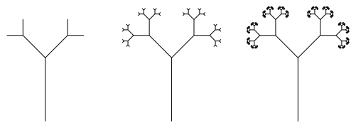
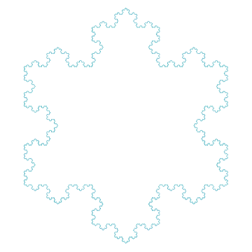
Day033Koch1b Thomas asked if it might be possible to keep the overall shape of the snowflake, but change the details at the edges. To discuss this possibility, let’s recall the algorithm for producing the snowflake (although this algorithm produces only one-third of the snowflake, so that three copies must be put together for the final image):

sf1(n):

if n = 0, then draw a line segment, otherwise:
sf1(n-1); turn -60; sf1(n-1); turn 120; sf1(n-1); turn -60; sf1(n-1)

This is “pseudocode” for drawing part of the snowflake n levels deep. The difficulty is that the segments are drawn only when n = 0. Thomas was wanting something different to happen, say, at level 3 and below in an algorithm which recursed 6 levels deep.

Then it occurred to me — there’s no reason the “otherwise” couldn’t be broken down into further cases: make the recursive call depend on the value n.

But in order to do this, I needed to use a different recursive call. What to use? Well, it happens that by slightly changing the angles in sf1, the snowflake undergoes a rotation by 30 degrees. Here is the pseudocode, along with the image.

sf2(n):

if n = 0, then draw a line segment, otherwise:
sf2(n-1); turn 120; sf2(n-1); turn -60; sf2(n-1); turn 120; sf2(n-1)

Day033Koch2

So how do we combine these fractals? As suggested earlier, break down the original “otherwise” clause. The following algorithm adds a “little” of the second snowflake to the first since the second algorithm is only called when n = 1.

new1(n):

if n = 0, then draw a line segment, otherwise:
if n = 1, sf2(n-1); turn 120; sf2(n-1); turn -60; sf2(n-1); turn 120; sf2(n-1)
else sf1(n-1); turn -60; sf1(n-1); turn 120; sf1(n-1); turn -60; sf1(n-1)

Here is the resulting fractal image (recursing 6 levels):

Day033Koch3

You can already see a difference. Now let’s try adding a little “more” of the second snowflake by using the second algorithm when n is 1 or 2, as shown below.

new2(n):

if n = 0, then draw a line segment, otherwise:
if n <= 2, sf2(n-1); turn 120; sf2(n-1); turn -60; sf2(n-1); turn 120; sf2(n-1)
else sf1(n-1); turn -60; sf1(n-1); turn 120; sf1(n-1); turn -60; sf1(n-1)

Day033Koch4

Going one level further — using the second algorithm when n is 1, 2, or 3 — produces the following curve. Day033Koch5

One level further yields:

Day033Koch6

And we’re done, since the next level will in fact give the rotated snowflake sf2(6) (although pieced together a little differently — but the resulting fractal is the same).

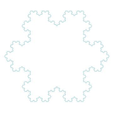
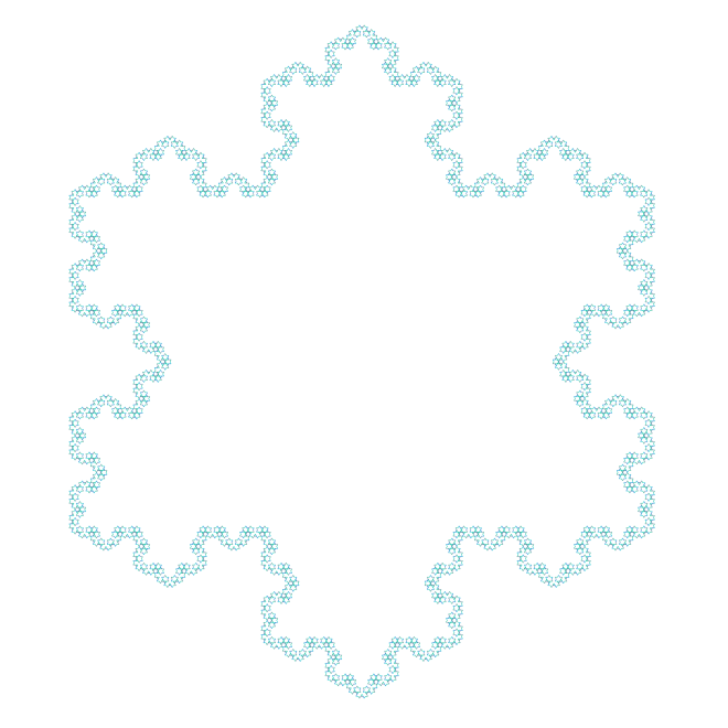
Now I’ll leave it up to you. There’s really so much to explore here. Here’s just one example. Adding just one additional call to sf2(n-1) after the last one in the algorithm produces the following image: Day033Koch7 Amazing, isn’t it? Such a small change results in a very different feel to the final image. And of course once smaller changes are made, there’s no reason to stop. Maybe branch into more than two fractal routines? Or maybe perform sf1 when n is odd, and sf2 when n is even. Or….

The only limitation, it seems, is one’s imagination. Comment if you create something interesing!

Creating Fractals IV: Results!

It has been a while since I wrote about making fractal images — and you might recall that I made several observations about how the images were drawn, but didn’t actually prove that these observations were valid in any general sense.

That has changed! A few weeks ago, I decided that it was time to bite the bullet. I had a concise way to describe what angles were chosen (see Creating Fractals, Day008, and Creating Fractals II: Recursion vs. Iteration, Day009), I accumulated a lot of empirical evidence that validated this description, and now it was time to prove it. I made a goal of solving the problem by the end of this semester.

It is amazing what a little determination can do! I went back to the code I wrote last October, stared at and studied countless sequences of angles and their corresponding images, and within a few days had a working hypothesis. Less than a week had gone by before I had a fairly complete proof. What I thought would take me an entire semester took me about a week.

In today’s post, I’ll talk about specific cases which directly relate to my previous blog posts. I won’t really prove anything here, but instead present the idea of the proof. When I write up the complete proof, I’ll post a link to the paper.

The main insight came from looking at sums of angles (mod 360). Let’s look at a specific example, using angles of 40 degrees and 60 degrees (both counterclockwise). These angles produce the following image:

$Day027fractal_40_60_1$

The angle sequence follows the pattern described in Creating Fractals II: 40, 60, 40, 40, 40, 60, etc., where the “40” occurs in position k if the highest power of 2 which divides k is even, and “60” occurs if this power is odd.

The arms in this figure have eight segments each; one such arm is highlighted below.

$Day027fractal_40_60_2$

Now let’s write the angle sums, starting with 0 since the first segment starts at the center and moved directly to the right. We get

Day027Table

The numbers at the top and left are for row/column reference only. We begin with 0, and 40, then add 60 to get 100, then add 40 more to get 140, etc. Once we hit 320 and need to add 60, we write 20 instead of 380 (since as far as angles go, 20 and 380 are equivalent). This is essentially saying that we are adding angles mod 360 (that is, using modular arithmetic).

These angle sums are the actual directions the lines are being drawn in the plane. You should be able to see the first two rows of this table clearly in the previous image — as you go around the first arm, your direction changes and points in the direction indicated by the appropriate sum in the table.

But notice the following interesting fact: each sum in Row 2 is exactly 180 degrees more than the corresponding sum in Row 1! What this means is as follows: once the first four segments are drawn, the next four are drawn pointing in the opposite directions. In other words, they geometrically “cancel out.” This means that after the first two rows, you’ll return to the origin (as seen above).

You can continue to follow along in the table and view the next arm being drawn, as shown below.

$Day027fractal_40_60_3$

This might seem “obvious” by looking at the table — but it is only obvious after you know how to draw the table. Then it’s easy! Even the mathematics is not all that difficult. I can’t emphasize enough, though, how using the computer to look at several (and more!) examples was a tremendous help in making progress towards how to arrange the table.

Now look at the “20” underlined at the beginning of Row 5. Because of the recursive pattern of the angles, this means that the next eight segments drawn will exactly repeat the second arm.

Just when do the arms repeat? The underlined angles (which indicate the direction the next eight segments are starting off) are the beginning of the sequence

0, 20, 20, 40, 60, 80, 80, 100, 100, 120, ….

If we look at the successive differences, we obtain the sequence

20, 0, 20, 20, 20, 0, 20, 0, 20, ….

But notice that this is the same pattern as the sequence of angles:

40, 60, 40, 40, 40, 60, 40, 60, 40, …

This means that the same pattern which indicates which angle to choose also determines which arms are redrawn. Really amazing!

The separation of 20 degrees between arms is just 60 – 40. In general, if d is the difference between the two angles, you need to take the greatest common divisor of d and 360, which is often abbreviated gcd(d, 360). But in this case, since 20 is already a factor of 360, you get the difference back.

Once you know the arms are separated by 20 degrees, you know that there are 360/20 = 18 arms in the final image.

As I mentioned, it is possible to prove all this — and more. Although we looked at a specific case, it is possible to make generalizations. For example, there were 8 segments in each arm — and 8 is a power of 2 (namely 3). But other powers of two are possible for the number segments in arms — 4, 32, 64, etc.

In addition, there is nothing special about degrees. Why divide a circle into 360 equal parts? You can divide the circle into a different number of parts, and still obtain analogous results.

The number of interesting images you can create, then, is truly astonishing. But the question still remains: have we found them all? In addition to all the images obtained by looking at arms whose segments number a power of two, it is possible to obtain more regular figures.

$Day027fractal_40_60_4$

Such images are obtained when both angles are the same. But other than this, I haven’t found any other types of figures.

So are there any others? Maybe. Maybe not. That’s part of the fun of doing mathematics — you just never know until you try. But I think this question will be a bit harder to answer. Is some enthusiastic reader tempted to find out? Perhaps all it takes is a little determination….