Imagifractalous – Creativity in Mathematics

Imagifractalous! 7: Fractal Binary Trees IV

Bridges 2017 is next week in Waterloo, Ontario, Canada! We’re all looking forward to it…Nick and his parents are also going, and I’ll get to see a lot of new friends I met last year in Finland.

In preparation, I’ve been creating a portfolio of binary and ternary trees. I’ve been coloring and highlighting the branches to make them easier to understand, so I thought I’d take the opportunity to share several of them. Mathematics just as it’s happening….

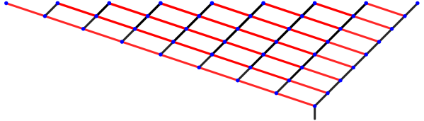
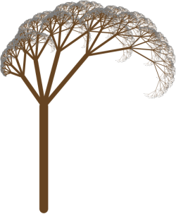
Here is an example of what I’m talking about.

2017-07-20-0is11v1

Recall that we’re generalizing the idea of “left” and “right” branches of a binary tree — rather that just rotating left or right (and possibly scaling), we’re allowing any affine transformation to correspond to “left” and “right.” In order to avoid any confusion, let’s refer to the transformations as “0” and “1.”

In the tree above, the 0 branches are shown in black, and the 1 branches in red. Notice that sometimes, the 0 branches seem to go to the right, other times, to the left. This is a common occurrence when you allow the branching to be determined by more general transformations.

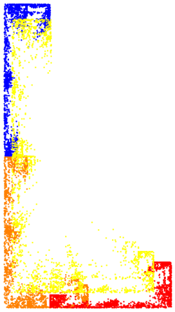
Here, you’ll notice that 0 and 11 take you to the same place — beginning with the trunk (the vertical black line at the right), if you follow one black branch, you’ll end up at the same blue node as you would if you followed two red branches. In fact, no matter what blue node you start at, following one black branch will always take you to the same place as following two red branches.

Here is not the place to go into too many details, but let me give you the gist of what we’re studying. If you denote the transformation which generates the black branches by $B_0$ and that which generate the red branches by $B_1,$ you will observe behavior like that in the above tree if

$B_0=B_1+B_1^2.$

Right now, most of the work I’m doing revolves around saying that I want to generate a tree with a certain property (like 0 and 11 going to the same node), and then solving the corresponding matrix equation to find interesting examples of trees with this property. Usually the linear algebra involved is fairly complicated — feel free to comment if you’d like to know more. As I said, this blog is not the place for all the details….

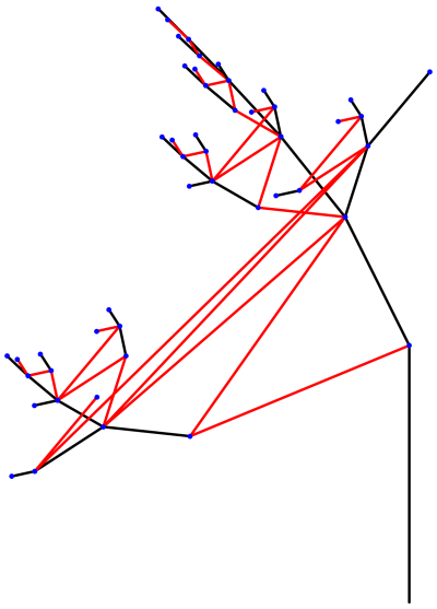
Below is another interesting example.

In this tree, 0 and 00 go to the same node. What this means in terms of branching is that there can never be two consecutive black branches (again, 0 is black and 1 is red) — taking the additional 0 branch leaves you in exactly the same place.

Note that for this property to hold, there is no restriction on what the 1 transformation can be. Above, the transformation $B_1$ is a scaled rotation by 60°. This is what produces the spirals of red branches emanating from the nodes of the tree.

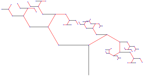
In this example, 0 and 01 go to the same node (0 is black, 1 is red). Implications for the tree are that the red branches zigzag back and forth, getting shorter with each iteration. Moreover, there aren’t any red branches drawn after a black branch (except the first time, off the end of the trunk of the tree). This is because 01 — taking a red branch after a black branch — takes you to the same place as 0, which is taking a black branch. In other words, the red branch doesn’t take you any further.

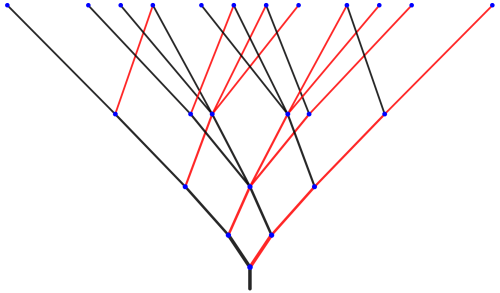
Here, 01 and 10 take you to the same node (again, 0 is black and 1 is red). This is easy to see — there are many quadrilaterals in the tree formed by alternating red and black branches. In addition, the iterations of this tree move progressively higher each time — so, for example, all the nodes at the top are at a depth of 4.

If you look at the number of new nodes at each level, you get a sequence which begins

2, 3, 6, 12, 24, 48, 96, 192, 384, 768, ….

After the second level, it seems that the number of new nodes doubles with each iteration. I say “seems” since it is generally very difficult to prove that such a relationship continues up arbitrarily many levels. Although it is easy to find the sequence of numbers of nodes for any tree using Mathematica, I have rigorous proofs of correctness for only three cases so far.

What makes the proofs so difficult? The following tree is another example of a case where 01 and 10 go to the same node.

2017-06-25-01is10v1

But the sequence of new nodes at each level is just 2, 3, 4, 5, 6, …. (This is one case I’ve rigorously proved.) The transformations $B_0$ and $B_1$ used to make this tree, in addition to forcing 01 and 10 to go to the same node, also have additional properties which force any two strings of the same length with the same number of 0’s (and therefore the same number of 1’s as well) to go to the same node. So to prove the sequence of nodes in the previous case is 2, 3, 6, 12, 24, 48, …, you need to say which strings take you to the same nodes, and prove that this pattern continues no matter how far you go up — and that there are no “surprise” coincidences of other nodes as you proceed.

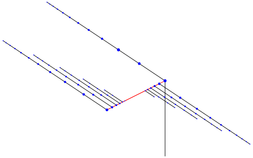
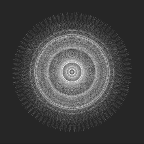
It is also possible to look at infinite strings going to the same node, as shown below. The linear algebra gets quite a bit more involved in these cases.

Here, 0 and 1 do in fact correspond to going left and right, respectively. The thicker black path corresponds to the string 011111…, that is, going left once, and then going to the right infinitely often, creating the spiral you see above. The thicker green path corresponds to alternating 10101010… infinitely often, creating a zigzag path which approaches exactly the same point as the black spiral does.

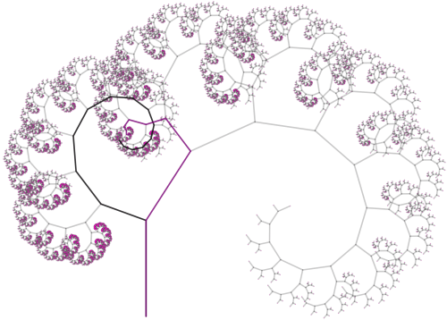
Here is another example, where the spiral 011111… (in black) approaches the same point as the infinite zigzag 100100100100… (in purple).

These are some of my favorite examples. But I should remark that once you know how to mathematically find transformations which produce trees with a desired property, it takes a lot of fiddling around to find aesthetically pleasing examples.

I hope these examples give you a better idea of the nature of our research. I’ll update you on Bridges when I get back, and let you know about any interesting comments other participants make about our trees. I leave on Wednesday, and will post pictures daily on my Twitter @cre8math if you’d like a daily dose of mathematical art!

Imagifractalous! 6: Imagifractalous!

No, the title of today’s post is not a typo….

About a month ago, a colleague who takes care of the departmental bulletin boards in the hallway approached me and asked if I’d like to create a bulletin board about mathematical art. There was no need to think it over — of course I would!

Well, of course we would, since I immediately recruited Nick to help out. We talked it over, and decided that I would describe Koch-like fractal images on the left third of the board, Nick would discuss fractal trees on the right third, and the middle of the bulletin board would highlight other mathematical art we had created.

I’ll talk more about the specifics in a future post — especially since we’re still working on it! But this weekend I worked on designing a banner for the bulletin board, which is what I want to share with you today.

BBoardBanner

I really had a lot of fun making this! I decided to create fractals for as many letters of Imagifractalous! as I could, and use isolated letters when I couldn’t. Although I did opt not to use a third fractal “A,” since I already had ideas for four fractal letters in the second line.

The “I”‘s came first. You can see that they’re just relatively ordinary binary trees with small left and right branching angles. I had already incorporated the ability to have the branches in a tree decrease in thickness by a common ratio with each successive level, so it was not difficult to get started.

I did use Mathematica to help me out, though, with the spread of the branches. Instead of doing a lot of tweaking with the branching angles, I just adjusted the aspect ratio (the ratio of the height to the width of the image) of the displayed tree. For example, if the first “I” is displayed with an aspect ratio of 1, here is what it would look like:

2017-04-16Tree1

I used an aspect ratio of 6 to get the “I” to look just like I wanted.

Next were the “A”‘s. The form of an “A” suggested an iterated function system to me, a type of transformed Sierpinski triangle. Being very familiar with the Sierpinski triangle, it wasn’t too difficult to modify the self-similarity ratios to produce something resembling an “A.” I also like how the first “A” is reminiscent of the Eiffel Tower, which is why I left it black.

I have to admit that discovering the “R” was serendipitous. I was reading a paper about trees with multiple branchings at each node, and decided to try a few random examples to make sure my code worked — it had been some time since I tried to make a tree with more than two branches at each node.

When I saw this, I immediately thought, “R”! I used this image in an earlier draft, but decided I needed to change the color scheme. Unfortunately, I had somehow overwritten the Mathematica notebook with an earlier version and lost the code for the original “R,” but luckily it wasn’t hard to reproduce since I had the original image. I knew I had created the branches only using simple scales and rotations, and could visually estimate the original parameters.

The “C” was a no-brainer — the fractal C-curve! This was fairly straightforward since I had already written the Mathematica code for basic L-systems when I was working with Thomas last year. This fractal is well-known, so it was an easy task to ask the internet for the appropriate recursive routine to generate the C-curve:

+45 F -90 F +45

For the coloring, I used simple linear interpolation from the RGB values of the starting color to the RGB values of the ending color. Of course there are many ways to use color here, but I didn’t want to spend a lot of time playing around. I was pleased enough with the result of something fairly uncomplicated.

For the “T,” it seemed pretty obvious to use a binary tree with branching angles of 90° to the left and right. Notice that the ends of the branches aren’t rounded, like the “I”‘s; you can specify these differences in Mathematica. Here, the branches are emphasized, not the leaves — although I did decide to use small, bright red circles for the leaves for contrast.

The “L” is my favorite letter in the entire banner! Here’s an enlarged version:

This probably took the longest to generate, since I had never made anything quite like it before. My inspiration was the self-similarity of the L-tromino, which may be made up of four smaller copies of itself.

2017-04-16Ltromino

The problem was that this “L” looked too square — I wanted something with a larger aspect ratio, but keeping the same self-similarity as much as possible. Of course exact self-similarity isn’t possible in general, so it took a bit of work to approximate is as closely as I could. I admit the color scheme isn’t too creative, but I liked how the bold, primary colors emphasized the geometry of the fractal.

The “O” was the easiest of the letters — I recalled a Koch-like fractal image I created earlier which looked like a wheel with spokes and which had a lot of empty space in the interior. All I needed to do was change the color scheme from white-on-gray to black-on-white.

Finally, the “S.” This is the fractal S-curve, also known as Heighway’s dragon. It does help to have a working fractal vocabulary — I knew the S-curve existed, so I just asked the internet again…. There are many ways to generate it, but the easiest for me was to recursively producing a string of 0’s and 1’s which told me which way to turn at each step. Easy from there.

So there it is! Took a lot of work, but it was worth it. I’ll take a photo when it’s actually displayed — and update you when the entire bulletin board is finally completed. We’ve only got until the end of the semester, so it won’t be too long….

Imagifractalous! 2: p-adic sequences

In Imagifractalous! 1, I talked about varying parameters in the usual algorithm for creating the Koch curve to produce a variety of images, and casually mentioned p-adic valuations. What happened was about a year after I began exploring these interesting images, I did a Google search (as one periodically does when researching new and exciting topics), and stumbled upon the paper Arithmetic Self-Similarity of Infinite Sequences.

It was there that I recognized the sequence of 0’s and 1’s I’d been using all along, and this sequence was called a 2-adic valuation (mod 2).

Here’s the definition: the p-adic valuation is the sequence such that the nth term in the sequence is the highest power of p which divides n. So the 2-adic valuation begins

0, 1, 0, 2, 0, 1, 0, 3, 0, 1, 0, 2, 0, 1, 0, 4, ….

Of course all terms with odd n are 0, and for the even n, you just look at the highest power of 2 dividing that even number. And you can take this sequence (mod 2), or mod anything you like.

I naturally did what any right-thinking mathematician would do — looked up p-adic sequences in the The On-Line Encyclopedia of Integer Sequences. Now it’s not that p-adic valuations are all that obscure, it’s just I had never encountered them before.

Of course there it was: A096268. And if you read through the comments, you’ll see one which states that this sequence can be used to determine the angle you need to turn to create the Koch snowflake.

I wasn’t particularly discouraged — this sort of thing happens all the time when exploring new mathematical ideas. You just get used to it. But something unexpected happened.

I starting experimenting with other p-adic valuations mod 2 (since I had two choices of angles), and found similar interesting behavior. Not only that, p didn’t have to be prime — any integer would do.

But most papers about p-adic valuations assumed p was prime. Why is that? If $\nu_p$ is a p-adic valuation and p is prime, it’s not hard to show that

$\nu_p(mn)=\nu_p(m)+\nu_p(n),$

an often-used property in developing a theory of p-adic valuations. But it only takes a moment to see that

$\nu_6(4)=0,\quad \nu_6(9)=0,\quad \nu_6(4\cdot9)\ne\nu_6(4)+\nu_6(9).$

Bad news for the p-adic theorists, but the fractal images couldn’t seem to care whether p was prime or not….

Beginning segment of a curve based on a 12-adic valuation.

So I didn’t plunge into researching p-adic valuations, since I needed a treatment which included p composite, which didn’t seem to be out there.

But here’s the neat part. Most of the work I’d done to prove something already known — that a 2-adic valuation (mod 2) could be used to produce a Koch curve — could be used to study generic p. So I was able to make fairly good progress in a relatively short amount of time, since I’d already thought about it a lot before. I suspect it would have taken me quite a bit longer if I’d just casually read about the 2-adic result rather than prove it myself.

The progress made was similar to that of the 2-adic case — number of segments in each arm in the symmetric case, how many solutions given a particular order of symmetry, and so forth.

Now my fractal brain was truly revved up! I enjoyed creating images using various p-adic valuations — the variety seemed another dimension of endless. So I started brainstorming about ways to even further diversify my repertoire of fractal images.

The first two weeks of November were particularly fruitful. Two ideas seemed to coalesce. The first revolved around an old unexplored question: what happened when you didn’t only change the angles in the algorithm to produce the Koch snowflake, but you also changed the lengths?

Of course this seemed to make the parameter space impossibly large, but I was in an adventurous mood, and the only thing at stake was a few moments with Mathematica generating uninteresting images.

Image based on a 3-adic valuation with different edge lengths.

But what I found was that if an image closed up with a particular symmetry, then as long as the sequence of edge lengths was appropriately periodic, the image with different edge lengths also closed up with the same order of symmetry!

This was truly mind-boggling at first. But after looking at lots of images and diving into the algorithm, it’s not all that improbable. You can observe that in the image above, segments of the same length occur in six different orientations which are 60 degrees apart, and so will ultimately “cancel out” in any final vector sum and take you right back to the origin.

Now I don’t have the precise characterization of “appropriately periodic” as yet, but I know it’s out there. Just a matter of time.

The second big idea at the beginning of November involved skimming through the paper on arithmetic self-similarity mentioned above. Some results discussed adding one sequence to another, and so I wondered: what if you added two p-adic sequences before taking their sum (mod 2)?

2016-11-22-8+64adic.png — Imaged based on adding 8-adic and 64-adic valuations with different edge lengths.

Well, preliminary results were promising only when the p-adic valuations involved were of the same power of some p, like in the image above (which also involves different edge lengths).

These ideas are only in a very preliminary stage — it’s the perennial problem of, well, waiting….. It may look liking adding 2-adic and 3-adic valuations doesn’t get you anywhere, but maybe that’s just because you need so many more iterations to see what’s actually happening. So there’s lots more to explore here.

Beginning segment of an image based on a 42-adic valuation.

So as the parameter space gets larger — mutliple different lengths, adding several different p-adic valuations — the variety becomes infinitely diverse, and the analysis becomes that much more involved.

But that makes it all the more intriguing. And it will be all the more rewarding when I finally figure everything out….

Imagifractalous! 1: How it all began.

September 2, 2015 — that was the day Thomas sent an email to the faculty in the math department asking if anyone was willing to help him learn something about fractals. And that was when it all began.

Now I’ve told this story in various forms over the past year or so on my blog, but I want to begin a thread along a different direction. I’d like to give a brief chronological history of my work with fractals, with an eye toward the fellow mathematician interested in really understanding what is going on.

I’ll be formal enough to state fairly precisely the mathematical nature of what I’m observing, so as to give the curious reader an idea of the nature of the mathematics involved. But I’ll skip the proofs, so that the discussion doesn’t get bogged down in details. And of course provide lots of pictures….

You might want to go back to read my post of Day007 — there is a more detailed discussion there. But the gist of the post is the question posed by Thomas at one of our early meetings: what happens when you change the angles in the algorithm which produces the Koch curve?

What sometimes happens is that the curve actually closes up and exhibits rotational symmetry. As an example, when the recursive routine

F +40 F +60 F +40 F

is implemented, the following sequence of segments is drawn.

Now this doesn’t look recursive at all, but rather iterative. And you certainly will have noticed something curious — some sequences of eight segments, which I call arms, are traversed twice.

All of this behavior can be precisely described — all that’s involved is some fairly elementary number theory. The crux of the analysis revolves around the following way of describing the algorithm: after drawing the nth segment, turn +40 degrees if the highest power of 2 dividing n is even, and turn +60 degrees if it’s odd. Then move forward.

I would learn later about p-adic valuations (this is just a 2-adic valuation), but that’s jumping a little ahead in the story. I’ll just continue on with what I observed.

What is also true is that the kth arm (in this case, the kth sequence of eight segments) is retraced precisely when the highest power of power of 2 dividing k is odd. This implies the following curious fact: the curve in the video is traced over and over again as the recursion deepens, but never periodically. This is because the 2-adic valuation of the positive integers isn’t periodic.

So I’ve written up some results and submitted them to a math journal. What I essentially do is find large families of angle pairs (like +40 and +60) which close up, and I can describe in detail how the curves are drawn, what the symmetry is, etc. I can use this information to create fractal images with a desired symmetry, and I discuss several examples on a page of my mathematical art website.

As one example, for my talks in Europe this past summer, I wanted to create images with 64 segments in each arm and 42-fold symmetry. I also chose to divide the circle in 336 parts — subdivision into degrees is arbitrary. Or another way of looking at it is that I want my angles to be rational multiples of $\pi,$ and I’m specifying the denominator of that fraction.

Why 336? First, I needed to make sure 42 divided evenly into 336, since each arm is then 8/336 away from the previous one (although they are not necessarily drawn that way). And second, I wanted there to be enough angle pairs so I’d have some choices. I knew there would be 96 distinct images from the work I’d already done, so it seemed a reasonable choice. Below is one of my favorites. The angles used here are 160 and 168 of the 336 parts the circle is divided into.

koch_336_6_160_168

Now my drawing routine has the origin at the center of the squares in the previous two images, so that the rotational symmetry is with respect to the origin. If you think about it for a moment, you’ll realize that if both angles are the same rational multiple of $\pi,$ you’ll get an image like the following, where one of the vertices of the figure is at the origin, but the center of symmetry is not at the origin.

$fractal_40_60_4$

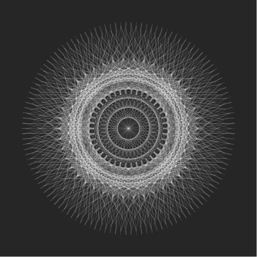
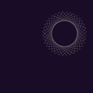
Of course it could be (and usually is!) the case that the curve does not close — for example, if one angle is a rational multiple of $\pi,$ and the other is an irrational multiple of $\pi.$ Even when they do close, some appealing results are obtained by cropping the images.

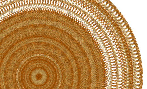
koch-60-254web

So where does this bring me? I’d like a Theorem like this: For the recursive Koch algorithm described by

F $\alpha_0$ F $\alpha_1$ F $\alpha_0$ F,

the curve closes up precisely when (insert condition on $\alpha_0$ and $\alpha_1$ ), and has the following symmetry (insert description of the symmetry here).

I’m fairly confident I can handle the cases where the center of symmetry is at the origin, but how to address the case when the center of symmetry is not the origin is still baffling. The only cases I’ve found so far are when $\alpha_0=\alpha_1,$ but that does not preclude the possibility of there being others, of course.

At this point, I was really enjoying creating digital artwork with these Koch-like images, and was also busy working on understanding the underlying mathematics. I was also happy that I could specify certain aspects of the images (like the number of segments in each arm and the symmetry) and find parameters which produced images with these features. By stark contrast, when I began this process, I would just randomly choose angles and hope for the best! I’d consider myself lucky to stumble on something nice….

So it took about a year to move from blindly wandering around in a two-dimensional parameter space (the two angles to be specified) to being able to precisely engineer certain features of fractal images. The coveted “if-and-only-if” Theorem which says it all is still yet to be formulated, but significant progress toward that end has been made.

But then my fractal world explodes by moving from 2-adic to p-adic. That for next time….