On Coding IV: Mathematica

In my last installment of “On Coding,” I talked more about functional proramming and how working with LISP so heavily influenced my coding in Mathematica.  To continue the thread, I’ll need to jump ahead on my timeline, since a lot of what I’ll say applies to my current use of Mathematica.  Then next time, I’ll need to jump back to my college days since I was also learning Postscript in parallel with LISP and Mathematica.

One nice feature of LISP and Mathematica interfaces is that they’re interpreters, meaning you interact directly with the kernel.  I can just type “3 + 2” and get a return value of 5, without needing to put the expression in a wrapper function.  This makes is easy to try out new functions.  And in Mathematica, there are thousands of functions — so lots to try out!

But aside from functional programming aspects, I think one fundamental advantage of using LISP or Mathematica is the fundamental data structure:  a list “(  )” in LISP, or “{  }” in Mathematica.  This is a fluid, untyped data structure, and is perhaps the most general way to store data.

In many languages, variables are typed.  That means if you want an array, you have to say what is in the array.  Is it an array of integers?  String?  Reals?  You can’t mix and match.

In Mathematica (and other languages as well, like Python), there are no restrictions as to what goes in a list.  So you can have a list like

{42, 3.1416, “Hello world!”, {0, 1, 2}},

and that would be no problem at all.

This is actually a very nice feature, but you do have to be careful.  If you try evaluating

Plus @@ {42, 3.1416, “Hello world!”, {0, 1, 2}},

you actually get

{45.1416 + “Hello World!”, 46.1416 + “Hello World!”, 47.1416 + “Hello World!”}!

The reason is that the “+” operator in Mathematica is overloaded, meaning it performs differently depending on what the arguments are.

The 42 + 3.1416 = 45.1416 is evaluated first.  Now a real can’t be added to a string, so Mathematics leaves the expression in an abstract form,

45.1416 + “Hello World!”,

without actually evaluating.  But when {0, 1, 2} is finally added, the “+” operator adds 45.1416 + “Hello World!” to each element of the list, and returns the resulting list.  Of course addition is commutative, so 0, 1, and 2 are added to the real part of the expression.

In a language like C++ or even Python, this would be unthinkable.  You’d get an error message right away.  But in Mathematica, all would be well — almost.  If you made a typo in your list of objects to add and Mathematica found a way to add them, you might get some rather bizarre behavior if that result were passed to some other function.  In other words, you’ve just got to be careful.

This fluidity makes creating graphics easy, in my opinion.  A graphics object is essentially a list of directives and objects, like

{Blue, Line[{{0,0}, {1,1}}], Red, Disk[{2,2}, 1]}.

Mathematica interprets this as follows.  First, make the stroke color Blue, and draw a line from (0,0) to (1,1).  Change the stroke color to Red, and then draw a disk of radius 1 centered at (2,2).

This loose structure makes creating graphics objects simple, as all you’re doing is building a list.  And that list contains a series of instructions about how to create an image.

There’s a slight drawback, for me at least.  I get frustrated sometimes when I program in a language like Python, where data structures enclosed in “[  ]” might be lists, tuples, or vectors, for example.  You often need to explicitly say what you want, as in using the function

vector([0, 1, 2]).

This is highly annoying to the Mathematica programmer, who thinks Python should be clever enough to figure it out….  So I find myself always looking up what type of argument is passed to a certain function to make sure I don’t get a runtime error.

Another advantage of using LISP and Mathematica, in my opinion, is that the return value of a function is the last statement executed.  This is a very nice feature — once you get used to it, you can’t image how you ever lived without it….

Let’s look at a simple example which takes advantage of this feature and uses some functional programming ideas.  Here’s the Python code:

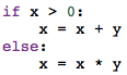
Nothing complicated going on here, just add two variables based on whether one of them is positive or not.  Here is the Mathematica code:

Yes, it’s really just one line!  The If statement returns the function “Plus” if the variable x is positive, and the function “Times” otherwise.  This return value can be immediately applied to the list containing x and y in order to carry out the desired operation.

Unless you’ve worked with a functional programming language before, this type of coding construct might seem a little strange.  But once you get used to thinking this way, you really can code more efficiently.

I also like that the decision about what function to used is very clearly based on whether the variable x is positive or not, since the If statement returns the name of a function.  Of course it’s clear in the Python code since the example is so simple, but the Mathematica code really drives the point home.

The one drawback for me is forgetting the “return” statement in Python all the time.  I’m so used to this feature in Mathematica that it’s automatic in my thinking about code.

The list structure and how return values are handled, in additional to the functional programming aspects, are the two features which most directly impact the way I write code in Mathematica.  But I can’t end this discussion without saying a few words about graphics.

I enjoy the absolute control you have about every feature in Mathematica.  You essentially have a blank slate, and can put just about anything you want anywhere you want.  I’ve never used a user interface to create graphics, and never will.

The reason is that you are often constrained by the available options with a GUI.  Not so in Mathematica.  Essentially, if you can conceive it, you can implement it.  It may take some time and a lot of code, but it can be done….

So that briefly summarizes my relationship with Mathematica, which is ongoing.  Next time, Postscript!