Digital Art II: End of Week 4

It’s hard to believe it’s been four weeks already!  Recall that we ended Week 2 with work on an Evaporation piece.  We’ll see examples of student work after a brief recap of Weeks 3 and 4 (Days 6–10).

In the past two weeks, we focused on affine transformations and their use in creating fractals with iterated function systems.  This was not intended to be a deep discussion of linear algebra, but a practical one — how affine transformations reflect the geomtetry of fractal images.

Days 6 and 7 were an introduction to the geometry of affine transformations.  I like to emphasize the geometry first, so I worked to find a way to simply and unambiguously describe an affine transformation geometrically.

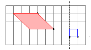
The blue square represents the unit square, and the red parallelogram the transformed square.  The filled-in/open black circles on the parallelogram represent how (0,0) and (1,0) are transformed, respectively.  Additionally, the pink fill in the parallelogram represents that fact that there is a flip (that is, the determinant of the linear part of the transformation is negative).  Strictly speaking, this coloring isn’t necessary, but I think it helps.

We then worked on writing the affine transformation in the form

We did this in the usual way, where the columns of the matrix represent where the unit basis vectors are transformed, and the vector added at the end is the translation from the origin.  These can all be read from the diagram, so that the picture above describes the affine transformation

To help in visualizing this in general, I also wrote a Sage worksheet which produces diagrams like the above picture given the parameters a—f.  In addition, I showed how the vertices of the parallelogram may be found algebraically by using the transformation itself, so this meant we could look at affine transformations geometrically and algebraically, as well as with the Sage worksheet.   (Recall that all worksheets/assignments may be found on the corresponding day on the course website.  In addition, I have included the code for the assignments for those interested.)

I explained several different types of affine transformations — translations, reflections, scalings, and shears.  On Day 8, we saw how to write the affine transformations which describe the Sierpinski triangle, and students got to play with creating their own fractals using the accompanying Sage worksheet.

On Day 9, I took about half the class to go through three of my blog posts on iterated function systems.  I emphasized the first spiral fractal discussed on Day035, paying particular attention to the rotation involved and matrix multiplication.

Most students weren’t familiar with trigonometry (recall the course has no prerequisites), so I just told them the formula for rotation matrices.  We briefly discussed matrix multiplication as function composition.  I gave them homework which involved some practice with the algebra of matrix multiplication.

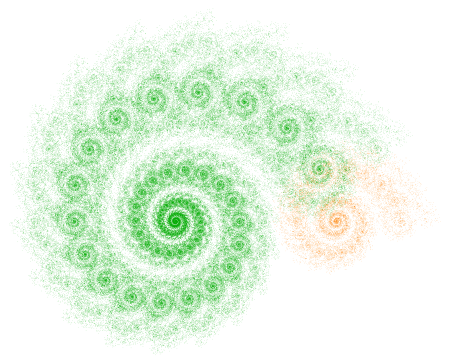
On Day 10, we began with going over some previous homework, and then looked at what transformations were needed to producing the fractal below (as practice for their upcoming homework).

We then engaged in the following laboratory exercise:  Create a fractal using two affine transformations.  For the first, rotate by 45 degrees, then scale the x by 0.6 and the y by 0.4, and finally move to the right 1.  For the second transformation, rotate 90 degrees clockwise, and then move up 1.

This was practice in going from a geometrical description to a fractal — they needed to perform the appropriate calculations, and then enter the data in the Sage worksheet and see if their fractal was correct (I gave them a link to the final image).

This turned out to be very challenging, as they were just getting familiar with rotations and matrix multiplication.  So we’ll need to finish during the next class.  I’ll also give them another similar lab exercise during the next class to make sure they’ve got it.

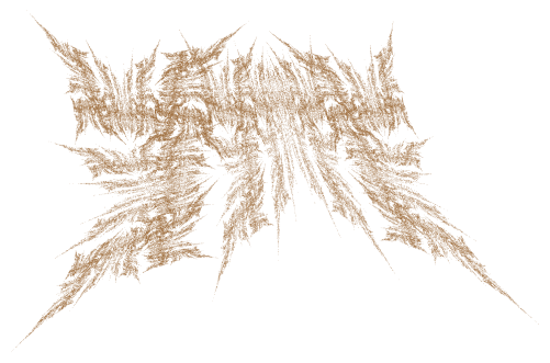
Last week’s digital art assignment was another success!  Again, I was very pleased with how creative my students were.  If you look back at the Sage worksheets, you’ll see that the class was working with color, texture, and color gradients (like my Evaporation piece).

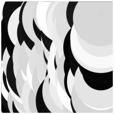
One student created a texture with a lot of movement by keeping the circles separate and using a wide range of gray tones.

Maddie took advantage of the fact that the algorithm draws the circles in a particular order to create a scalloped texture.  This happens when the circles are particularly large, since the circles are drawn in a linear fashion, creating successive overlap.

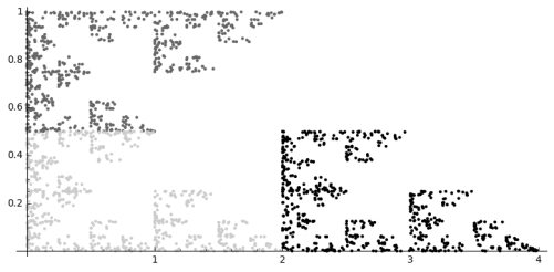
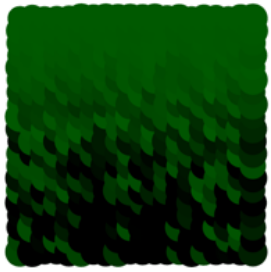
Another student also used this overlapping feature with a color gradient.  He describes his piece as follows:

This piece is what I like to call “The Hedge” as it reminds me a lot of those tall square hedges that are in mansions. It’s as if the light is hitting the top of the hedge and dispersing down into the shadows and thickness of the leaves. I especially like the leafy effect the overlapping circles give.

Finally, Madison experimented with altering the dimensions of the grid to create a different feel.

She thought that making the image wider made the evaporation effect more pronounced.

These are just some examples of how students in my Mathematics and Digital Art course take ideas I give them and make them their own.  They are always asking how they can incorporate one effect or another into their work, and Nick and I are glad to oblige by helping out with a little code.

As I strive to keep my posts a consistent length, I won’t be able to share all the images I’d like to this week.  So I’ll be posting additional images on my Twitter feed, @cre8math.  Follow along if you’d like to see more!