Color I: Opacity and Josef Albers

What do you see?

Looks like a pink square on top of a purple square.  But after hearing a talk about Josef Albers’ work at Bridges 2016 a few weeks ago, I realized there is more than one way to look at this image.

Maybe the square is actually more red, but transparent — so that the purple showing through makes it pink.  Or maybe the pink square is behind the purple square, and it’s the purple square which is transparent.  Or maybe the purple square isn’t a square at all, but a frame — that is, a square with a hole in it!

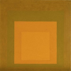
This first post in a series on color will explore this apparently simple figure.  The ultimately goal will be to analyze images in Josef Albers’ series Homage to the Square. But as mentioned last week, James Mai found that there are 171 possible combinations of opaqueness, transparency, frames, and squares in this series!  So we’ll start with a basic example.

But first, we have to understand how opacity works in computer graphics.  We’ve used RGB colors in several posts so far, but rarely mentioned opacity.  When this is included, the color system is referred to as RGBA, where the “A” represents the opacity (or alternatively, the transparency), which is also sometimes called the alpha.  A value of means that the color is completely transparent, so it doesn’t affect the image at all, while a value of means the color is completely opaque, meaning you can’t see through it at all.

As an example, in the series below, the squares have RGB values of (0.2, 0, 1.0), and A values of 0.25, 0.5, 0.75, and 1.0 (going from left to right).

But these squares could also have been created without any transparency at all!  What this means is that if you include transparency/opacity, there are many different ways to specify a color that appears on your screen, not just one.  So in an Albers’ piece with four squares, where all of them may have some degree of transparency, the analysis can be quite difficult.

Next, we have to understand how the opacity is used to create the colors you see.  If color has opacity and is on top of a color the apparent or observed color is then

If you thought to yourself, “Oh, it’s linear interpolation again!”, you’d be right!  In other words, the observed color is a linear combination of the transparent color and the background color.

Keep in mind that is an idealized situation.  It is very difficult to make a correspondence with how we “actually” see.  If you were looking at an object throught a square of colored glass — maybe sunglasses — there would be concerns about the distance between the glass and the object, multiple lighting sources, etc.  For now, we just want to understand the mathematics of using opacity in computer graphics.

Another complication arises in considering the following two squares — a pure red square on top of a pure blue square.

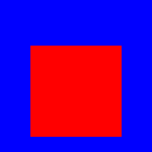
In this case, it is impossible that the red square has any degree of transparency.  If it did, some of the blue would show through.  If the red square had a transparency of our linear interpolation formula would give an apparent color of

This means if there were any transparency at all, there would be a Blue component of the observed color, which is not possible since Red has RGB values of (1,0,0).  So before you go about calculating opacity, you’ve got to decide if it’s even possible!

Let’s start with the purple square.

What color could this square be, with what transparency?  Let’s call the color and the opacity  Since the background (screen color) is white, we use

To assess what the color “looks like,” you’d go to PhotoShop and use the eyedropper tool, for example — or another other application which allows you to point to a color and get the RGB values.  In this case, you’d get (0.6, 0.5, 1.0).  Basically, what you get with such tools are RGB values, assuming an opacity of

But of course we’re wondering what is possible if the opacity is not 1.  If we denote by we get

which simplifes to

This gives us three equations in four unknowns, which makes sense — we know the answer is likely not unique since it may be possible to create the square using different opacities.

Note that the third equation is

which when rearranged gives us

Of course cannot be 0, or we wouldn’t see anything!  This means which makes sense since if we’re interpolating between and 1, the only way to get a result of 1.0 would be if

What about the other equations,

Solving them, we get

Keep in mind that the and values must all be between 0 and 1.  So we must at least have

to guarantee that all values are positive.  Further, observe that for any value between 0.5 and 1 (inclusive), we have that the numerators of both color values are less than the demoninators, and are therefore less that 1.

So this means that the purple square may be created using the color values

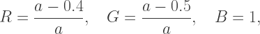
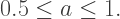
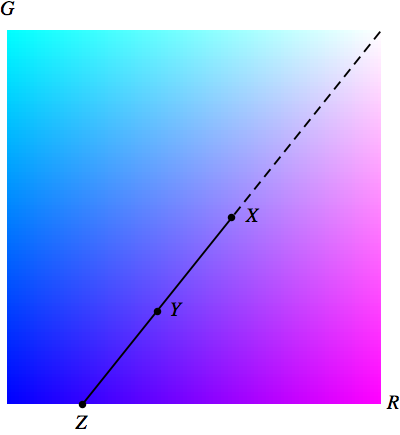
as long as the opacity satisfies  This is illustrated graphically below, where the solid line segment represents all possible colors for the square.

Here, the horizontal axis is the Red component and the vertical axis is the Green component.  Since we observed earlier that the Blue component must alwas be 1, the lower-left corner would be (0,0) in RG space (Blue), and the upper-right corner would be (1,1) (White).  When we obtain the point X with RGB values (0.6, 0.5).  This makes sense, since we observed the color to have RGB values (0.6, 0.5, 1.0).

When we obtain the point Y with coordinates (0.4, 0.25) in RG space.  This means the purple square could be obtained using RGB values of (0.4, 0.25, 1.0) and opacity

And when we obtain the point Z with coordinates (0.2, 0) in RG space.  This means the purple square could be obtained using RGB values of (0.2, 0, 1.0) and opacity 0.5.

Note that even though Y is  halfway between X and Z in RG space, the value is not halfway between 0.5 and 1.0.  This is because of the in the denominators in the fractions above giving solutions for R and G.

There’s a nice geometrical interpretation of this picture, too.  If one color is an interpolation of two others, it must lie on the segment joining those two others.  So we need all colors C such that X is on the segment between C and (1,1).  This is just that part of RG space which is a continuation of the line starting at (1,1) and going past X.

Now we could have just used this geometrical idea from the beginning — but I wanted to work out the mathematics so you could see how to use the definition of opacity to solve color problems.  And of course sometimes the geometry is not so obvious, so you need to start with the algebraic definition.

So working with opacity isn’t too difficult as long as you understand what your computer is doing.  In the next post on Color, we’ll tackle the issue of the pink square….