Now that the paper Nick and I wrote on binary trees was accepted for Bridges 2017 (yay!), I’d like to say a little more about what we discovered. I’ll presume you’ve already read the first Imagifractalous! post on binary trees (see Day077 for a refresher if you need it).
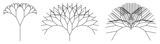
Recall that in that post, I discussed creating binary trees with branching ratios which were 1 or larger. Below are three examples of binary trees, with branching ratios less that 1, equal to 1, and larger than 1, respectively.
It was Nick’s insight to consider the following question: how are trees with branching ratio r related to those with branching ratio 1/r? He had done a lot of exploring with graphics in Python, and observed that there was definitely some relationship.
Let’s look at an example. The red tree is a binary tree with branching ratio r less than one, and the gray tree has a branching ratio which is the reciprocal r. Both are drawn to the same depth.
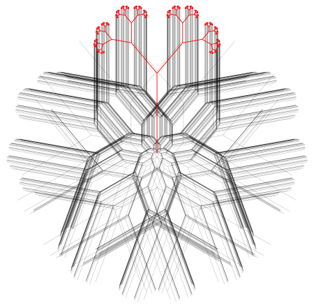
Of course you notice what’s happening — the leaves of the trees are overlapping! This was happening so frequently, it just couldn’t be coincidence. Here is another example.
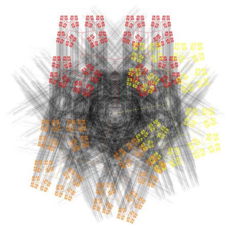
Notice how three copies of the trees with branching ratio less than one are covering some of the leaves of a tree with the reciprocal ratio.
Now if you’ve ever created your own binary trees, you’ll likely have noticed that I left out a particularly important piece of information: the size of the trunks of the trees. You can imagine that if the sizes of the trunks of the r trees and the 1/r trees were not precisely related, you wouldn’t have the nice overlap.
Here is a figure taken from our paper which explains just how to find the correct relationship between the trunk sizes. It illustrates the main idea which we used to rigorously prove just about everything we observed about these reciprocal trees.
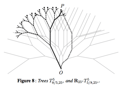
Let’s take a look at what’s happening. The thick, black tree has a branching ratio of 5/8, and a branching angle of 25°. The thick, black path going from O to P is created by following the sequence of instructions RRRLL (and so the tree is rendered to a depth of 5).
Now make a symmetric path (thick, gray, dashed) starting at P and going to O. If we start at P with the same trunk length we started with at O, and follow the exact same instructions, we have to end up back at O.
The trick is to now look at this gray path backwards, starting from O. The branches now get larger each time, by a factor of 8/5 (since they were getting smaller by a factor of 5/8 when going in the opposite direction). The size of the trunk, you can readily see, is the length of the last branch drawn in following the black path from O to P. This must be (5/8)5 times the length of the trunk, since the tree is of depth 5.
The sequence of instructions needed to follow this gray path is RRLLL. It turns out this is easy to predict from the geometry. Recall that beginning at P, we followed the instructions RRRLL along the gray path to get to O. When we reverse this path and go from O to P, we follow the instructions in reverse — except that in going in the reverse direction, what was previously a left turn becomes a right turn, and vice versa.
So all we need to do to get the reverse instructions is to reverse the string RRRLL to get LLRRR, and then change the L‘s to R‘s and the R‘s to L‘s, yielding RRLLL.
There’s one important detail to address: the fact that the black tree with branching ratio 5/8 is rotated by 25° to make everything work out. Again, this is easy to see from the geometry of the figure. Look at the thick gray path for a moment. Since following the instructions RRLLL means that in total, you make one more left turn than you do right turns, the last branch of the path must be oriented 25° to the left of your starting orientation (which was vertical). This tells you precisely how much you need to rotate the black tree to make the two paths have the same starting and ending points.
Of course one example does not make a proof — but in fact all the important ideas are contained in this one illustration. It is not difficult to make the argument more general, and we have successfully accomplished that (though this blog is not the place for it!).
If you look carefully at the diagram, you’ll count that there are exactly 10 leaves in common with these two trees with reciprocal branching ratios. There is some nice combinatorics going on here, which is again easy to explain from the geometry.
You can see that these common leaves (illustrated with small, black dots) are at the ends of gray branches which are oriented 25° from the vertical. Recall that this specific angle came from the fact that there was one more L than there were R‘s in the string RRLLL.
Now if you have a sequence of 5 instructions, the only way to have exactly one more L than R‘s is to have precisely three L‘s (and hence two R‘s). And the number of ways to have three L‘s in a string of length 5 is just
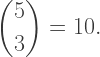
Again, these observations are easy to generalize and prove rigorously.
And where does this take us?
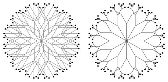
On the right are 12 copies of a tree with a braching ratio of r less than one and a branching angle of 30°, and on the left are 12 copies of a tree with a reciprocal branching ratio of 1/r, also with a branching angle of 30°. All are drawn to depth 4, and the trunks are appropriately scaled as previously discussed.
These sets of trees produce exactly the same leaves! We called this the Dual Tree Theorem, which was the culmination of all these observations. Here is an illustration with both sets of trees on top of each other.
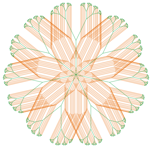
As intriguing as this discovery was, it was only the beginning of a much broader and deeper exploration into the fractal world of binary trees. I’ll continue a discussion of our adventures in the next installment of Imagifractalous!
