I love hyperbolic trigonometry. I always include it when I teach calculus, as I think it is important for students to see. Why?
- Many applications in the sciences use hyperbolic trigonometry; for example, the use of Laplace transforms in solving differential equations, various applications in physics, modeling population growth (the logistic model is a hyperbolic tangent curve);
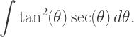
- Hyperbolic trigonometric substitutions are, in many instances, easier than circular trigonometric substitutions, especially when a substitution involving
 or
or  is involved;
- Students get to see another form of trigonometry, and compare the new form with the old;
- Hyperbolic trigonometry is fun.
OK, maybe that last reason is a bit of hyperbole (though not for me).
Not everyone thinks this way. I once had a colleague who told me she did not teach hyperbolic trigonometry because it wasn’t on the AP exam. What do you say to someone who says that? I dunno….
In any case, I want to introduce the subject here for you, and show you some interesting aspects of hyperbolic trigonometry. I’m going to stray from my habit of not discussing things you can find anywhere online, since in order to get to the better stuff, you need to know the basics. I’ll move fairly quickly through the introductory concepts, though.
The hyperbolic cosine and sine are defined by

I will admit that when I introduce this definition, I don’t have an accessible, simple motivation for doing so. I usually say we’ll learn a lot more as we work with these definitions, so if anyone has a good idea in this regard, I’d be interested to hear it.
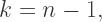
The graphs of these curves are shown below.
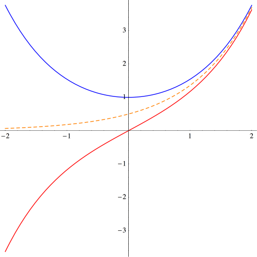
The graph of  is shown in blue, and the graph of
  is shown in red. The dashed orange graph is
  which is easily seen to be asymptotic to both graphs.
Parallels to the circular trigonometric functions are already apparent:  is an even function, just like
 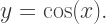 Similarly, is odd, just like
Another parallel which is only slight less apparent is the fundamental relationship

Thus,  lies on a unit hyperbola, much like
  lies on a unit circle.
While there isn’t a simple parallel with circular trigonometry, there is an interesting way to characterize and  Recall that given any function
  we may define

to be the even and odd parts of respectively. So we might simply say that and are the even and odd parts of  respectively.
There are also many properties of the hyperbolic trigonometric functions which are reminiscent of their circular counterparts. For example, we have

and

None of these are especially difficult to prove using the definitions. It turns out that while there are many similarities, there are subtle differences. For example,

That is, while some circular trigonometric formulas become hyperbolic just by changing  to and
  to
to  sometimes changes of sign are necessary.
These changes of sign from circular formulas are typical when working with hyperbolic trigonometry. One particularly interesting place the change of sign arises is when considering differential equations, although given that I’m bringing hyperbolic trigonometry into a calculus class, I don’t emphasize this relationship. But recall that is the unique solution to the differential equation

Similarly, we see that is the unique solution to the differential equation

Again, the parallel is striking, and the difference subtle.
Of course it is straightforward to see from the definitions that  and
and  Gone are the days of remembering signs when differentiating and integrating trigonometric functions! This is one feature of hyperbolic trigonometric functions which students always appreciate….
Another nice feature is how well-behaved the hyperbolic tangent is (as opposed to needing to consider vertical asymptotes in the case of ). Below is the graph of 
The horizontal asymptotes are easily calculated from the definitions. This looks suspiciously like the curves obtained when modeling logistic growth in populations; that is, finding solutions to

In fact, these logistic curves are hyperbolic tangents, which we will address in more detail in a later post.
One of the most interesting things about hyperbolic trigonometric functions is that their inverses have closed formulas — in striking contrast to their circular counterparts. I usually have students work this out, either in class or as homework; the derivation is quite nice, so I’ll outline it here.
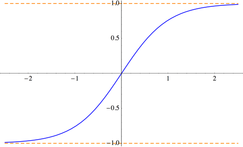
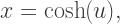
So let’s consider solving the equation  for
for  Begin with the definition:

The critical observation is that this is actually a quadratic in 
All that is necessary is to solve this quadratic equation to yield

and note that  is always negative, so that we must choose the positive sign. Thus,

And this is just the beginning! At this stage, I also offer more thought-provoking questions like, “Which is larger,  or
or  These get students working with the definitions and thinking about asymptotic behavior.
Next week, I’ll go into more depth about the calculus of hyperbolic trigonometric functions. Stay tuned!


 where it crosses the x-axis at
  we simply retain the
  term and substitute the root
  into the other terms, getting

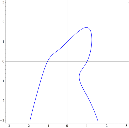
 (the U-shaped piece, since the sideways U-shaped piece involves writing
  as a function of
  ) is
) is  as shown below.
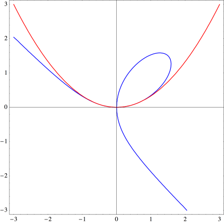

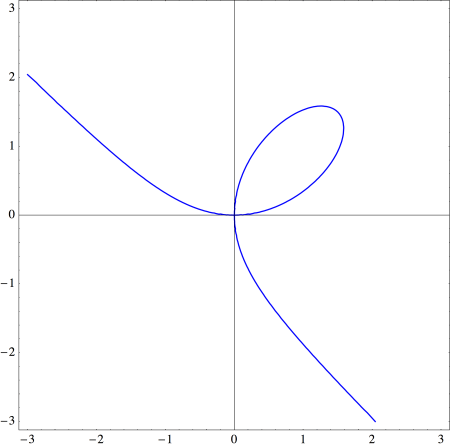
 and so rewrite the equation for the Folium of Descartes by using the substitution
  which results in
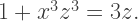
 we have
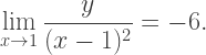
  giving us a good quadratic approximation at the origin.
 looking at the curve

 with
with  yet to be determined. This results in
 we have
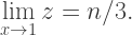
 Thus, in our case with
  we see that
  is a good approximation to the curve near the origin. The graph below shows just how good an approximation it is.
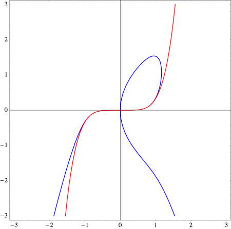

 which results in
 here. But if we move the
  to the other side and factor, we get
 to obtain
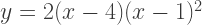
 And sure enough, the line
  does the trick:
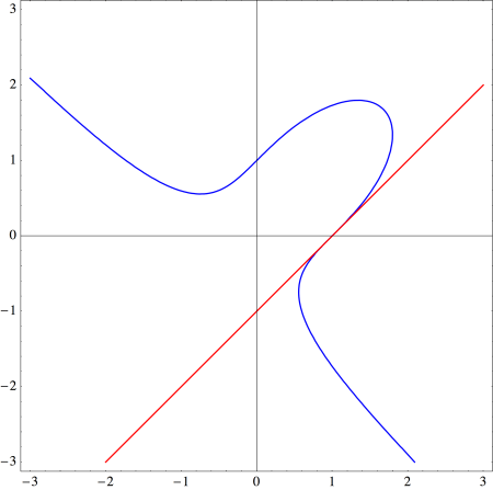


 This results in
 is even, since there is always a root at
  in this case. Here, we make the substitution
  move the
  resulting in
 is a factor of
  so we have

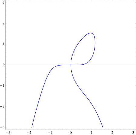
 as well! This is a curious coincidence, for which I have no nice geometrical explanation. The case when
  is illustrated below.
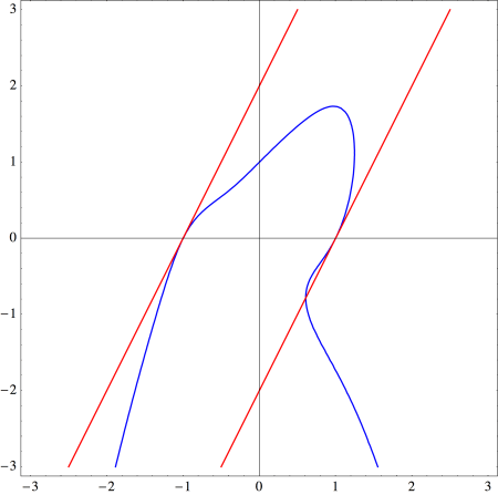

 Today, we’ll look at some more examples, and then derive the product, quotient and chain rules.

 as small as we like, and so approximate by considering
  as the sum of an infinite series:
 We first factor the denominator:
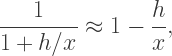
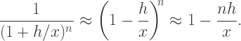


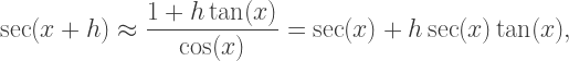
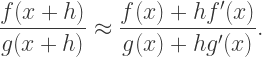
 so we replace each factor with its linear approximation:


 (or perhaps
  ). I have found that there is just no way to convincingly motivate this step. Yes, those of us who have seen it crop up in various forms know to try such tricks, but the typical first-time student of calculus is mystified by that mysterious step. Using linear approximations, there is absolutely no mystery at all.


 and
and  but note that this involves using the chain rule to differentiate
  or (2) the mysterious “adding and subtracting the same expression” in the numerator. Using linear approximations avoids both.
 is differentiable, it is also continuous, so this poses no real problem. Yes, perhaps there is a little hand-waving here, but in my opinion, no rigor is really lost.
 is differentiable, then
  exists, and so we can make
  as small as we like, so the “
 ” term acts like the “


 Writing the limit in this way, we see that
  as a function of
  is linear in

 This is not difficult to prove.
 It’s easy to see that
 to the limit. So the coefficient of


 and see how it looks using this rewrite. We first write
 and
and  near
near  we have
 But how do we justify the approximation
 ? We need
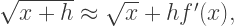

 so must be the coefficient on the right, so that
 Then we have
 we have
  and so we can replace to get
 then
then  is small (as small as we like), and so we can consider
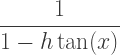


 occurs quadratically.
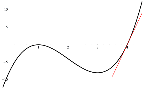
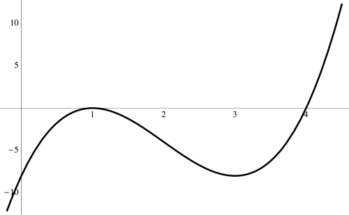
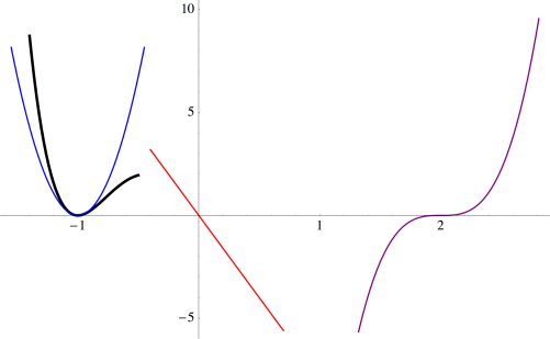
 the graph passes through the x-axis like a line — and we see a linear factor of
  in our polynomial.
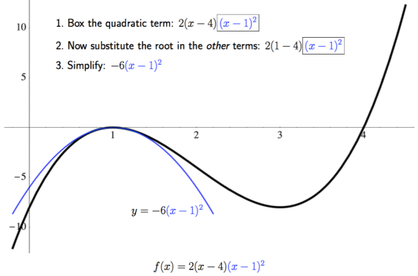
 and substitute the root,
  near the root
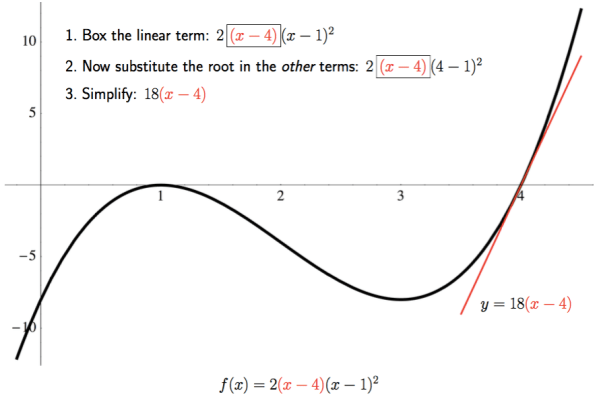
 substitute
  in the remaining terms of the polynomial, and then simplify. Thus, the line
  best describes the behavior of the graph of the polynomial as it passes through the x-axis. Again, note the scale on the axes.
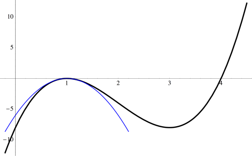
 Begin by sketching the three approximations near the roots of the polynomial. This slide also shows the calculation for the cubic approximation.
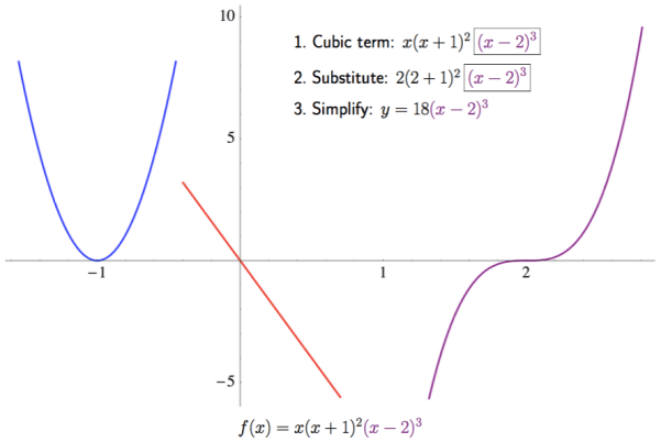

 Of course you’d need to plot a few points to know just where to start and end; this just shows how you would use the approximations near the roots to help you sketch a graph of a polynomial.
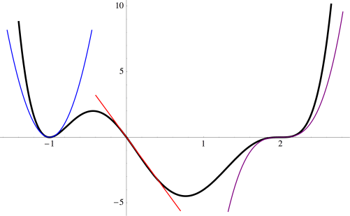
 near the root
  Given what we’ve just been observing, we’d guess that the best approximation near
  would just be
 match at
  derivatives of both of these functions at
  will always be a factor — since at most
  term to completely “disappear.”
 at
at  What about the
  When a derivative of
  is taken, that means one factor of
  we also get
  and
and 

