Day139 – Creativity in Mathematics

As I mentioned last week, I am a fan of emphasizing the idea of a derivative as a linear approximation. I ended that discussion by using this method to find the derivative of $\tan(x).$ Today, we’ll look at some more examples, and then derive the product, quotient and chain rules.

Differentiating $\sec(x)$ is particularly nice using this method. We first approximate

$\sec(x+h)=\dfrac1{\cos(x+h)}\approx\dfrac1{\cos(x)-h\sin(x)}.$

Then we factor out a $\cos(x)$ from the denominator, giving

$\sec(x+h)\approx\dfrac1{\cos(x)(1-h\tan(x))}.$

As we did at the end of last week’s post, we can make $h$ as small as we like, and so approximate by considering $1/(1-h\tan(x))$ as the sum of an infinite series:

$\dfrac1{1-h\tan(x)}\approx1+h\tan(x).$

Finally, we have

$\sec(x+h)\approx\dfrac{1+h\tan(x)}{\cos(x)}=\sec(x)+h\sec(x)\tan(x),$

which gives the derivative of $\sec(x)$ as $\sec(x)\tan(x).$

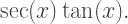
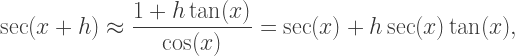
We’ll look at one more example involving approximating with geometric series before moving on to the product, quotient, and chain rules. Consider differentiating $x^{-n}.$ We first factor the denominator:

$\dfrac1{(x+h)^n}=\dfrac1{x^n(1+h/x)^n}.$

Now approximate

$\dfrac1{1+h/x}\approx1-\dfrac hx,$

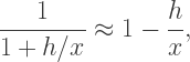
so that, to first order,

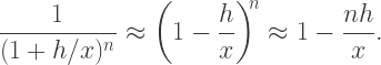
$\dfrac1{(1+h/x)^n}\approx \left(1-\dfrac hx\right)^{\!\!n}\approx 1-\dfrac{nh}x.$

This finally results in

$\dfrac1{(x+h)^n}\approx \dfrac1{x^n}\left(1-\dfrac{nh}x\right)=\dfrac1{x^n}+h\dfrac{-n}{x^{n+1}},$

giving us the correct derivative.

Now let’s move on to the product rule:

$(fg)'(x)=f(x)g'(x)+f'(x)g(x).$

Here, and for the rest of this discussion, we assume that all functions have the necessary differentiability.

We want to approximate 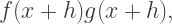$f(x+h)g(x+h),$ so we replace each factor with its linear approximation:

$f(x+h)g(x+h)\approx (f(x)+hf'(x))(g(x)+hg'(x)).$

Now expand and keep only the first-order terms:

$f(x+h)g(x+h)\approx f(x)g(x)+h(f(x)g'(x)+f'(x)g(x)).$

And there’s the product rule — just read off the coefficient of $h.$

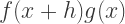
There is a compelling reason to use this method. The traditional proof begins by evaluating

$\displaystyle\lim_{h\to0}\dfrac{f(x+h)g(x+h)-f(x)g(x)}h.$

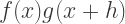
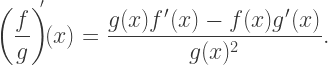
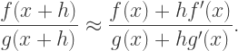
The next step? Just add and subtract $f(x)g(x+h)$ (or perhaps $f(x+h)g(x)$ ). I have found that there is just no way to convincingly motivate this step. Yes, those of us who have seen it crop up in various forms know to try such tricks, but the typical first-time student of calculus is mystified by that mysterious step. Using linear approximations, there is absolutely no mystery at all.

The quotient rule is next:

$\left(\dfrac fg\right)^{\!\!\!'}\!(x)=\dfrac{g(x)f'(x)-f(x)g'(x)}{g(x)^2}.$

First approximate

$\dfrac{f(x+h)}{g(x+h)}\approx\dfrac{f(x)+hf'(x)}{g(x)+hg'(x)}.$

Now since $h$ is small, we approximate

$\dfrac1{g(x)+hg'(x)}\approx\dfrac1{g(x)}\left(1-h\dfrac{g'(x)}{g(x)}\right),$

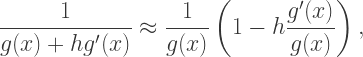
so that

$\dfrac{f(x+h)}{g(x+h)}\approx(f(x)+hf'(x))\cdot\dfrac1{g(x)}\left(1-h\dfrac{g'(x)}{g(x)}\right).$

Multiplying out and keeping just the first-order terms results in

$\dfrac{f(x+h)}{g(x+h)}\approx f(x)g(x)+h\dfrac{g(x)f'(x)-f(x)g'(x)}{g(x)^2}.$

Voila! The quotient rule. Now usual proofs involve (1) using the product rule with $f(x)$ and $1/g(x),$ but note that this involves using the chain rule to differentiate $1/g(x);$ or (2) the mysterious “adding and subtracting the same expression” in the numerator. Using linear approximations avoids both.

The chain rule is almost ridiculously easy to prove using linear approximations. Begin by approximating

$f(g(x+h))\approx f(g(x)+hg'(x)).$

Note that we’re replacing the argument to a function with its linear approximation, but since we assume that $f$ is differentiable, it is also continuous, so this poses no real problem. Yes, perhaps there is a little hand-waving here, but in my opinion, no rigor is really lost.

Since $g$ is differentiable, then $g'(x)$ exists, and so we can make $hg'(x)$ as small as we like, so the “ $hg'(x)$ ” term acts like the “ $h$ ” term in our linear approximation. Additionally, the “ $g(x)$ ” term acts like the “ $x$ ” term, resulting in

$f(g(x+h)\approx f(g(x))+hg'(x)f'(g(x)).$

Reading off the coefficient of $h$ gives the chain rule:

$(f\circ g)'(x)=f'(g(x))g'(x).$

So I’ve said my piece. By this time, you’re either convinced that using linear approximations is a good idea, or you’re not. But I think these methods reflect more accurately the intuition behind the calculations — and reflect what mathematicians do in practice.

In addition, using linear approximations involves more than just mechanically applying formulas. If all you ever do is apply the product, quotient, and chain rules, it’s just mechanics. Using linear approximations requires a bit more understanding of what’s really going on underneath the hood, as it were.

If you find more neat examples of differentiation using this method, please comment! I know I’d be interested, and I’m sure others would as well.

In my next installment (or two or three) in this calculus series, I’ll talk about one of my favorite topics — hyperbolic trigonometry.

Tag: Day139

Calculus: Linear Approximations, II