On Coding V: Postscript

It has been a while since my last On Coding installment — I talked about Mathematica and functional programming.  Now its time to talk about one of my favorite programming languages:  Postscript!

Chronologically, we’re back in my undergraduate days, around sophomore year.  Recall that means no laptops, no slick user interfaces, no real windows environments like we know today.  This meant if you wanted to play around wtih computer graphics, you had to go to a computer lab and write code.  Postscript was the language of choice.

And get this.  The only way to see if you wrote your code correctly was to print out your graphics.  No fancy clicking your mouse and having the image rendered on your screen.  This meant debugging wasn’t so easy….

Two important features of Postscript are that it’s a stack-based language, and the notation is postfix — meaning the arguments come before the function call.  Just like my HP-15C programmable calculator, which is still functioning perfectly despite being over thirty years old.  It’s my go-to calculator when I want to make quick calculations.

I won’t go into detail here, since I discussed these two features at length in my Day037 blog post, Fractals VIII: PostScript Programming.  Feel free to go back and refresh your memory if you need to….

What I will discuss today are the two primary things I use Postscript for now:  iterated function systems and L-systems.

OK, I won’t really discuss iterated function systems as far as the algorithm is concerned…I’ve talked a lot about that before.  But what’s significant is that’s when I started getting hooked on fractals.  I had read about IFS in a paper by Michael Barnsley (before his famous Fractals Everywhere was written) just a few years after Mandelbrot’s The Fractal Geometry of Nature was first published.  Fractals weren’t so well-known at the time, but they were making quite a buzz in the mathematical community.

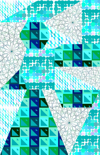
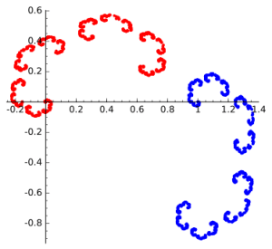
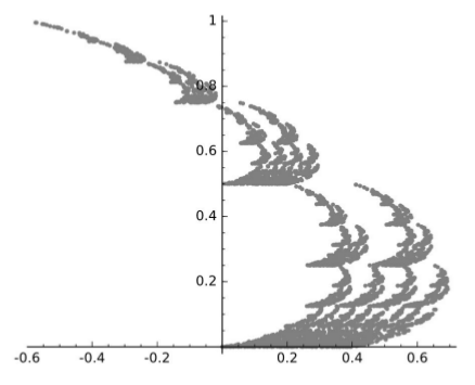
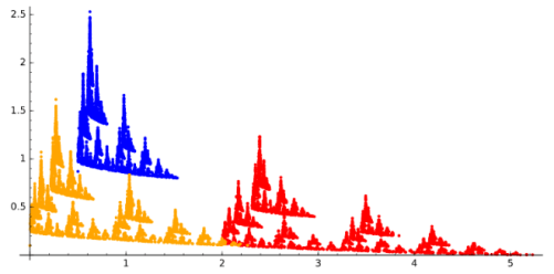
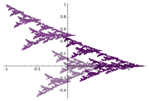
What was really neat was that I could make my own fractals in Postscript.  I was really struck by the wide variety of images you could make with just two affine transformations.  My favorite is still The Beetle.

Beetle2

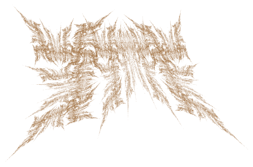
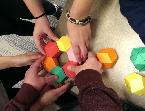
Now this particular image didn’t get rendered in Postscript until much later (my files are dated 1998), but the seeds were well-planted.  And fortunately, by then, there were nice GUIs so I didn’t have to rely on printing each image to see what it looked like….  I still use my old Postscript code to teach IFS occasionally, as I did with Thomas.

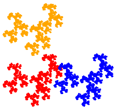
The other significant use of Postscript is in modeling L-systems (I’ve talked about these before, here is a nice Wikipedia page on the subject).  In particular, I implemented basic turtle graphics routines so I could imitate many of the well-known algorithms for creating fractals like the Koch and dragon curves.

Of course these algorithms could be implemented in any programming language.  But I didn’t have access to Mathematica at the time, I loved Postscript, and it was open source.  So it was a natural choice for me.

For the graphics programmer, there are a few particularly useful functions in Postscript, gsave and grestore.  These functions save and restore (respectively) what is called the graphics state.  In other words, if you are creating a graphical object, and would like to create another and return where you left off, you would invoke gsave, go do your other bit, and then use grestore to return where you left off.  Like a stack for graphics.

What this does is save all the parameters which influence how graphics are drawn — the current origin, rotation of axes, line thickness, color, dash pattern for lines, etc.  And there are a lot of such parameters possible in Postscript.

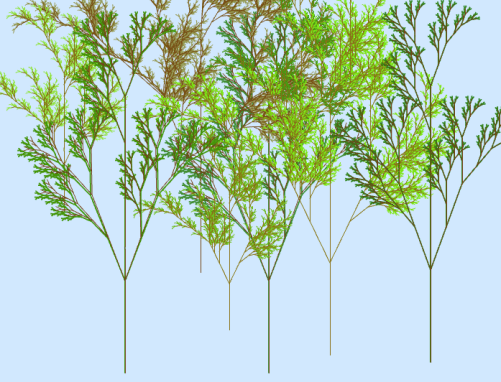
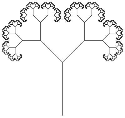
And while you might not think this is a really interesting feature, it’s great for working with L-systems, especially bracketed L-systems.  You might recall that a very basic binary tree is represented by the bracketed L-system

T(s)\rightarrow F(s)\,  [\,  +\,  T (r s)] \, [ \,-\, T(r s)].

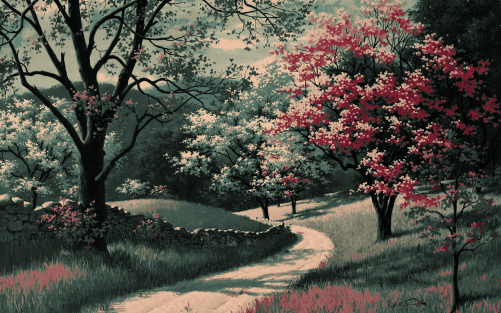
Basically, this means that a tree T is drawn first by moving forward some length s.  Remember where you are (“[“), then, turn left some given angle, and then draw a tree whose beginning segment has length rs, where r is less than 1, so that the left branch is a self-similar version of the whole tree.  Finish that tree (“]”), and go back to where you were. Then repeat on the right-hand side.  Here is a simple example with a branching angle of 45 degrees, and a branching ratio of 0.58.

2017-01-02binarytree.png

You might have guessed the punch line by now:  use gsave for “[” and grestore for “].”  Really nice!  There are a few other subtleties to take care of, like remembering the depth as you go along, but the gsave and grestore functions essentially make implementing bracketed L-systems fairly easy in Postscript.

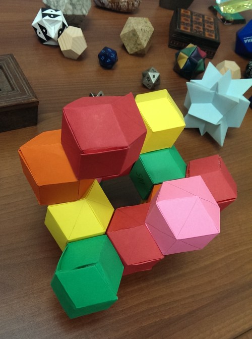
While I now use Postscript primarily for IFS and L-systems today, I’ve had other adventures with Postscript over the years.  Before they were easily available online in other places, I used Postscript to create dozens of nets for making polyhedra, such as the net for the rhombic dodecahedron shown below.

rhdodeca

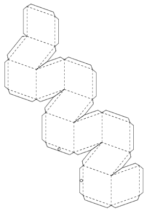
I had taught a course on polyhedra and geodesic structures for many years, so it was convenient to be able to make nets for classroom use.

I also played with designing fonts for a while (though I think those files are gone forever), and enjoyed designing stationery as well.  Here was one of my favorites.

pianokeys

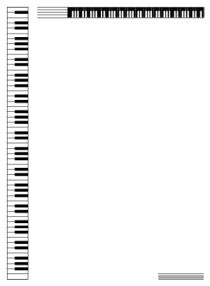
I just printed this motif on some nice paper, and used it to write letters — back in the day when people actually wrote letters!  It was fun experimenting with graphic design.

True, not many people program in Postscript now, since there are so many other options for producing graphics.  But I do always encourage students to dabble for a bit if they can.  Programming in Postscript gets you thinking in postfix and also thinking about stacks.  And while you may not use these concepts every day when programming, it’s good to have them in your coding arsenal.  Gives you more options.

In the next installment, I’ll talk about markup languages — LaTeX and HTML.  Until then!

Digital Art VIII: The End.

Yes, Mathematics and Digital Art is officially over.  Personally, this has been one of the most enjoyable courses I’ve taught, but also one of the more challenging.  From the initial course proposal — begun in November 2015! — to the Final Projects, it seems there was always something unexpected popping up.  But in a good way, since these surprises often involved such things as writing code for a student’s project, or helping a student incorporate a creative aspect into a digital artwork which I had not previously considered.

As I mentioned last week, the last assignment was to write a final Response Paper about the course.  Students had many good things to say, but also made some suggestions for improvement.

I feel like now, though, especially through the talks we were given from other artists, that my scope of the word “art” has broadened. The realm of digital art is so much wider than I could have imagined and includes a lot more mediums than I would have thought.

After completing this course, I realize that the world of art is even vaster, with so many areas still left unexplored or underexplored.

Wow!  I was so glad to see how the course broadened students’ perspectives.  Some students also mentioned the presentations on Bridges papers in this regard — how they were able to learn about many diverse topics in a brief amount of time.  They got a small taste of what it’s like to go to a Bridges conference….

As I had hoped, many students’ perspectives on mathematics changed during the course.  I’ll let the students speak for themselves.

Overall, I really enjoyed the class. Through high school, math was complicated and boring, but this class made me appreciate math in a different way, and I enjoyed learning about coding and digital art.

After this course, I definitely think about math differently, because now I know how it can be used to figure out shapes and layers and colors that I can use in my art. I also think differently about art, because before this course, I had only really done traditional art, and had no idea about any digital art besides using a tablet to draw with instead of a pencil. This course has really opened my mind to what I think art can be, and definitely how it can be created in different ways.

As with most classes, I learned a lot of significant things, but this class really taught me how to push beyond my boundaries and comfort zones. Learning about fractals and affine transformations were mathematically the most difficult part for me, but without those chapters I probably wouldn’t have sharpened my basic math skills….

I felt the coding part of the course was pitched at about the right level.

I soon realized that even though I had no background in code the material was explained and taught so that anyone could understand it.

But some  students commented that they would like to go into more depth as far as programming is concerned.

And one student even decided to minor in computer science!

Best of all, this class is part of the reason why I decided to declare a minor in computer science. It is something I have been considering as I have always had an interest in the subject, but I feel this class had really helped fuel that interest and give me the final nudge I needed.

Most students remarked about how much they loved learning to make movies in Processing, and how the small class size really helped them in terms of their personal learning experience.  The class was just nine students, and I had Nick to help me out — so I felt I really got to know the students.  Not a luxury I’ll always have….

Aside from focusing more on code, some students commented on how we didn’t really use the few weeks on polyhedra anywhere else in the course.  Yes, I wanted to give them some exposure to three-dimensional geometry without having to spend the time developing the mathematics of a three-dimensional Cartesian coordinate system.  But it seems this was just too disjointed from the natural flow.

I think a good substitute would be to discuss L-systems for these two weeks instead.  There are two advantages here.  First, L-systems are another really neat way to create fractals, and the class responded very positively when I gave my Bridges talk on L-systems and Koch curves.  And second, this would give a few more weeks when we could discuss coding, especially recursion.  In general, recursion is a difficult topic to teach — but teaching recursion in the context of computer graphics might really help the learning process.

I also asked Nick if he’d say a few words about his experience with the course.

I was very excited to work with Professor Matsko on Math and Digital Art, I think we both caught on a while back that the great flexibility I’ve found within the math department to support creative interests can be shared with other students. Also the instant gratification that we were finding from programming was really picking up. When communication from generated images was profoundly more efficient than any attempt to explain with words, it was clear that we had to invite more people to the conversation.

What I think has been so powerful following my discovery of programming – and what I hope I left with the students – is the ability to paste mathematical notation for very specific thoughts directly into the computer so that I can just look at what those thoughts literally mean. This continues to be the best way that I’ve found to meet and greet interesting new patterns and behaviors. Ultimately I think this is extremely natural and that the students caught on quite well: curious how a fractal might react? Poke it and find out!

Some areas definitely saw unexpected challenges, but once we got their mathematical comfort zones lined up with the curriculum the enthusiasm was excellent. My favorite part was definitely helping students let their imaginations fill the newly available parameter space. It was really great that we had a small class size, too – the two of us walking around made the perfect environment for any question to be asked during open days when they worked on self-directed projects. And it really felt like success to observe students becoming fixed on a single idea of what they wanted to create, whether or not they knew anything about how they would create it.

Overall I may have learned more than the students and was very surprised by the deeper understanding that begins to build after explaining to the masses. I would be very interested in assisting a course again!

As long as enough students enroll, I’ll be teaching Mathematics and Digital Art again next semester!  I won’t be reporting as frequently as I did this first semester, but expect updates every month or so….  Who knows what creative ideas next semester’s students will come up with?

Digital Art VII: Final Projects!

It’s hard to believe that the semester has finally come to an end!  And I must say that Mathematics and Digital Art was one of most enjoyable courses I’ve ever taught.  I’ll summarize my thoughts in a later reflective post, but today I’d like to showcase my students’ Final Projects.  There really was some exceptional work — but I’ll let the images speak for themselves.

Many students built upon the work we did earlier in the semester. Safina used several different elements we explored during the course.  In addition, she researched turtle graphics in Python to incorporate additional elements (those with lines emanating from a central point).

SM-MathProjectFinal.png


A few students especially enjoyed the work we did with color and Josef Albers, and created projects around different ways to contrast colors.  Andrew created many variations on a triangular theme.

screen-shot-2016-11-20-at-7-02-02-pm

He took this idea further, and went so far as to combine different triangles in composite images.

Hexagon-01.png

Julia, on the other hand, experimented with other geometrical objects.  She played with having colors interact with each other, and created the following image.  Although it may not look like it, the two center circles are in fact exactly the same color!

jn-capture7

Two students were interested in image processing, and worked closely with Nick to learn how to use the appropriate Python libraries in order to work with uploaded images.  Madison’s work focused on sampling pixels in an image and replacing them with larger circles to create an impressionistic effect.  She found that using a gray background gave the best results.

MJ-Screen Shot 2016-11-30 at 9.51.23 PM.png


Lucas also worked with image processing.  He began by choosing a fairly limited color palette.  Then for each pixel in his image, he found the color on his palette “nearest” the color of that pixel (using the usual Euclidean distance on the RGB values), and then adjusted the brightness.  The image below is one example illustrating this approach.

LA-Screen Shot 2016-12-04 at 11.42.53 PM.png


Two students worked with textures we experimented with earlier in the semester to create pieces like Evaporation.  Maddie wanted to recreate a skyline of Dubai (photo from the Creative Commons).

mc-dubaiskyline

She picked out particular elements to emphasize in her work.  You can clearly see the tall buildings and lit windows in a screenshot of her movie.

MC-Screen Shot 2016-12-02 at 9.26.26 AM.png


Sharon was interested in working with some of Dali’s paintings, creating impressionistic images by mimicking Dali’s color palette.  Here is her interpretation of The Elephants.

sa-screen-shot-2016-12-11-at-1-28-20-pm

Although we only touched on L-systems briefly in class, Ella wanted to focus on them in her project.  Nick also worked closely with her to create different effects.  Here is a screenshot from one of her movies.

ek-screen-shot-2016-12-11-at-1-33-30-pm

She was able to create some interesting effects by just slightly altering the parameters to L-systems which created trees and superimposing the new L-system on top of the original.  This gave some depth to the trees in her forest.

And one student decided to revisit Iterated Function Systems, but this time using nonlinear transformations in a variety of different ways.  Here is one of her images.

af-screen-shot-2016-12-04-at-7-51-12-pm
So you can see the wide range of projects students undertook!  This typically happens when you give students the freedom to choose their own direction.  I was also inspired by the enthusiasm of some of the students’ presentations.  They really got into their work.

The last assignment was to write a final Response Paper about the course.  The prompt was the same as that for the Response Paper I assigned midway through the course, so I’m curious to see if their attitudes have changed.  I’ll talk about what I learn in next week’s post!


Digital Art VI: End of Week 14

The last three weeks have been very intense!  The main focus has been on laboratory work, both with Processing and Final Projects.

Week 12 began with another round of Presentations on papers from past Bridges conferences.  This proved to be successful again — with topics ranging from geometrical furniture to zippergons to maps of Thomas More’s Utopia.  We all learned something new!

The time not spent on Presentations that week was devoted to working on projects.  Students were finding their stride, and their ideas were really beginning to take shape.

Two students were interested in image processing, so Nick has been working with them.  The initial problem was that doing anything in Sage involving image processing was just too slow — you’re code is essentially sent to a remote server, executed, and the results sent back.  Since we’re using the free version, this means performance is unpredictable and far too slow for computation-heavy tasks.

So Nick helped with installing Python, finding image processing packages, etc.  This process always takes a lot longer than you imagine, but eventually all issues were resolved.

While Nick was working on image processing, I was helping others.  One student was really interested in using L-systems — one of my favorite geometrical topics recently!   But all my work with Thomas involved code written in Postscript and Mathematica.  Which meant I had to rewrite it in Python.

This proved to be quite a bit trickier than I thought.  The student was looking at The Algorithmic Beauty of Plants, and was interested in modeling increasingly complex L-systems.  First, the simplest type, like that used to generate the Koch curve.  Next came bracketed L-systems, and then bracketed L-systems with multiple rules.  I did finally get all these to work; I intend to clean up the code and share it in a future post.

Week 13 was devoted entirely to Processing and project work.  I started the week with introducing a few new ideas.  What really inspired the class were the mouseX and the mouseY variables.  When your mouse is in screen space, the mouseX and mouseY variables contain the location of your mouse.  So you can put an object where the mouse is, or have the x-coordinate of the mouse in some way determine the color or the size of the object.  The possibilities are virtually endless.

Here’s a sample movie made with this technique.

Since the code is just a few lines long, it won’t take long to explain.  Here is the complete program:

mouseanddot

The drawPoint function will draw a point centered at the position of the mouse.  But in addition to those coordinates, the function takes an addition argument:  float(mouseX)/500.  This argument is 0 at the left edge of the screen, and 1 at the right edge.  (Recall the need for “float,” since otherwise Python will perform integer division and give 0 for any number less than 500.)

So the stroke command uses the parameter p to determine how much red is in the color specification.  When p is 0, there is no red, so the dot is black.  And when p is 1, the dot is red.  I used “p**0.4” as an illustration that interpolation need not be linear — the exponent of p determines how quickly or slowly the dot gets brighter as you move the mouse to the right.  Of course the dot also gets larger as you move your mouse to the right, as is clear by the strokeWeight function call.

I showed this example as I introduced the movie project.  Their assignment was to make a movie — anything they wanted to try.  The complete prompt is given on Day 34 of the course website, but I’ll give the gist of it here.  The main goal was to have students use linear interpolation in at least four different ways in their movie.  Of course they could use nonlinear interpolation if they wanted to, but it wasn’t required.

There was no length requirement — it’s easy to make a movie longer by adding more frames.  Just be creative!  Interpolation is a very useful tool in making movies and animations, and has a mathematical basis as well.  So I wanted that to be the focus of the project.  I also had them write a brief narrative about their use of interpolation.

This is Andrew’s movie.  You can clearly see the use of interpolation here in different ways.  It was also nice to see the use of trigonometry to calculate the centers of the dots.


Ella was interested in L-systems, and so Nick spent some time working with her on Python code during his weekly office hours.  Here is what she created.


Lucas wanted to use some interaction with the mouse, and he also had the idea of the sun setting as you moved the mouse down the screen.  Watch how the fractal clouds move with the location of the mouse as well.


So you can see how varied the use of interpolation was!  The students really enjoyed having control over the possible special effects, and created a wide range of interesting features in their movies.

That takes us to Week 14.  On Monday, we had a guest speaker come in, Chamberlain Fong.  I met him in Finland at Bridges this summer, only to find out he lives the next neighborhood over in San Francisco!  He gave a very interesting talk about taking pictures with a spherical or hemispherical camera lens, and the issues involved in printing the pictures.

The problem is essentially the same as creating a map of the globe — making a sphere flat.  There will always be distortion, but you have some control over what type of distortion.  You can keep angles the same, or areas the same — or some combination of the two.  And as these cameras keep getting cheaper, there will be a growing interest in making your spherical photos look realistic.

And although we had class on Wednesday, some students had already left for Thanksgiving Break.  So Nick and I were available to help on an open lab day.  Most of the students actually showed up, and we had a productive day working on movies (which were due Wednesday) and projects.

The next (and final!) post on Mathematics and Digital Art will survey the students’ Final Projects, so stay tuned!

On Coding IV: Mathematica

In my last installment of “On Coding,” I talked more about functional proramming and how working with LISP so heavily influenced my coding in Mathematica.  To continue the thread, I’ll need to jump ahead on my timeline, since a lot of what I’ll say applies to my current use of Mathematica.  Then next time, I’ll need to jump back to my college days since I was also learning Postscript in parallel with LISP and Mathematica.

One nice feature of LISP and Mathematica interfaces is that they’re interpreters, meaning you interact directly with the kernel.  I can just type “3 + 2” and get a return value of 5, without needing to put the expression in a wrapper function.  This makes is easy to try out new functions.  And in Mathematica, there are thousands of functions — so lots to try out!

But aside from functional programming aspects, I think one fundamental advantage of using LISP or Mathematica is the fundamental data structure:  a list “(  )” in LISP, or “{  }” in Mathematica.  This is a fluid, untyped data structure, and is perhaps the most general way to store data.

In many languages, variables are typed.  That means if you want an array, you have to say what is in the array.  Is it an array of integers?  String?  Reals?  You can’t mix and match.

In Mathematica (and other languages as well, like Python), there are no restrictions as to what goes in a list.  So you can have a list like

{42, 3.1416, “Hello world!”, {0, 1, 2}},

and that would be no problem at all.

This is actually a very nice feature, but you do have to be careful.  If you try evaluating

Plus @@ {42, 3.1416, “Hello world!”, {0, 1, 2}},

you actually get

{45.1416 + “Hello World!”, 46.1416 + “Hello World!”, 47.1416 + “Hello World!”}!

The reason is that the “+” operator in Mathematica is overloaded, meaning it performs differently depending on what the arguments are.

The 42 + 3.1416 = 45.1416 is evaluated first.  Now a real can’t be added to a string, so Mathematics leaves the expression in an abstract form,

45.1416 + “Hello World!”,

without actually evaluating.  But when {0, 1, 2} is finally added, the “+” operator adds 45.1416 + “Hello World!” to each element of the list, and returns the resulting list.  Of course addition is commutative, so 0, 1, and 2 are added to the real part of the expression.

In a language like C++ or even Python, this would be unthinkable.  You’d get an error message right away.  But in Mathematica, all would be well — almost.  If you made a typo in your list of objects to add and Mathematica found a way to add them, you might get some rather bizarre behavior if that result were passed to some other function.  In other words, you’ve just got to be careful.

This fluidity makes creating graphics easy, in my opinion.  A graphics object is essentially a list of directives and objects, like

{Blue, Line[{{0,0}, {1,1}}], Red, Disk[{2,2}, 1]}.

Mathematica interprets this as follows.  First, make the stroke color Blue, and draw a line from (0,0) to (1,1).  Change the stroke color to Red, and then draw a disk of radius 1 centered at (2,2).

This loose structure makes creating graphics objects simple, as all you’re doing is building a list.  And that list contains a series of instructions about how to create an image.

There’s a slight drawback, for me at least.  I get frustrated sometimes when I program in a language like Python, where data structures enclosed in “[  ]” might be lists, tuples, or vectors, for example.  You often need to explicitly say what you want, as in using the function

vector([0, 1, 2]).

This is highly annoying to the Mathematica programmer, who thinks Python should be clever enough to figure it out….  So I find myself always looking up what type of argument is passed to a certain function to make sure I don’t get a runtime error.

Another advantage of using LISP and Mathematica, in my opinion, is that the return value of a function is the last statement executed.  This is a very nice feature — once you get used to it, you can’t image how you ever lived without it….

Let’s look at a simple example which takes advantage of this feature and uses some functional programming ideas.  Here’s the Python code:

pythonsnippet

Nothing complicated going on here, just add two variables based on whether one of them is positive or not.  Here is the Mathematica code:

mmasnippet

Yes, it’s really just one line!  The If statement returns the function “Plus” if the variable x is positive, and the function “Times” otherwise.  This return value can be immediately applied to the list containing x and y in order to carry out the desired operation.

Unless you’ve worked with a functional programming language before, this type of coding construct might seem a little strange.  But once you get used to thinking this way, you really can code more efficiently.

I also like that the decision about what function to used is very clearly based on whether the variable x is positive or not, since the If statement returns the name of a function.  Of course it’s clear in the Python code since the example is so simple, but the Mathematica code really drives the point home.

The one drawback for me is forgetting the “return” statement in Python all the time.  I’m so used to this feature in Mathematica that it’s automatic in my thinking about code.

The list structure and how return values are handled, in additional to the functional programming aspects, are the two features which most directly impact the way I write code in Mathematica.  But I can’t end this discussion without saying a few words about graphics.

I enjoy the absolute control you have about every feature in Mathematica.  You essentially have a blank slate, and can put just about anything you want anywhere you want.  I’ve never used a user interface to create graphics, and never will.

The reason is that you are often constrained by the available options with a GUI.  Not so in Mathematica.  Essentially, if you can conceive it, you can implement it.  It may take some time and a lot of code, but it can be done….

So that briefly summarizes my relationship with Mathematica, which is ongoing.  Next time, Postscript!

Digital Art V: End of Week 11

It’s been an exciting three weeks in Mathematics and Digital Art!  We began Week 9 after our Fall break with a talk by Carlo Sequin.  Here’s Carlo with one of his sculptures at the University of California, Berkeley.

imag3969

I met Carlo through the Bridges conferences; he currently sits on the Board.  Since he’s so close by, I thought it would be great to have him visit my class.

His talk centered around the computer graphics programs he wrote in order to design sculptures like the one you see in the picture above.  Carlo included several different parameters, allowing an incredible variety of images to be generated.

Then he focused on a few of his sculptures and described the design process from conception to final sculpture.  He even remarked how he got lucky once — he and his team forgot to measure the width of the door they needed to take the sculpture through, and it fit with just a few inches to spare….

Friday, Day 24, was our first Project day.  Students’ ideas were still somewhat vague — they did have to write a Proposal, but still didn’t have a clear direction.  We made some progress, though the next Project day helped quite a bit more.

On Monday, Day 25, we dived into working with Processing.  I kept in mind the comments from students’ response papers which I mentioned in my previous post — they really wanted to learn more about code.

Now coding is a precision endeavor, as there is no room for error as far as syntax is concerned.  So after working through a simple example, I presented them with the following movie.

Admittedly it’s not a blockbuster…but their lab work was to duplicate this movie as precisely as possible.  I gave them a basic template (see the May 2016 archives for the start of a six-part series on Processing which I used as a basis for their lab work), but they didn’t just have to tweak numbers — they also had to add new elements.

The main mathematical tool involved was linear interpolation, which we went over in some detail in class.  The next class, I had them work on recreating the following movie.

This proved a bit more challenging.  Some students at first thought there was a rotation involved — but it’s just linear interpolation again, on a somewhat larger scale.  Here are the prompts I gave them:

  • the screen is 500 x 500 pixels;
  • the dots are always 25 pixels from the edge;
  • the colors are the standard red, green, blue, and orange;
  • the smaller dots are 100 pixels wide, and the larger ones are 200 pixels wide.

The main challenge was working in screen space, since they needed to calculate the exact centers of the circles.  Of course students progressed at different rates, and they were finally getting the main point — you can use linear interpolation to morph any aspect of an image which depends on a numerical parameter.  As a mathematician, I was used to thinking along these lines all the time, but it’s a concept that takes a while to really sink in if it’s new.

Friday, Day 27, was our next project day.  We worked at fleshing out more details of the students’ various projects.  Two students wanted to explore image processing, so Nick continued working with them to download the appropriate packages and get Python installed on their computers.  Such projects are never as easy as they sound, but Nick did get everything to work.

While he was doing that, I circulated with the other studets, discussing their projects and answering a few questions about making movies, if they had them.  It was a productive day, and everyone left class with a much clearer idea of their project than they had the week before.

On Monday, we continued our work with Processing.  I went through an example from my earlier blog posts — making a movie which morphs a Sierpinski triangle — in some detail, explaining it line by line.  Again, the most challenging part was converting from user space to screen space.  A fractal which fit in a unit square had to be scaled and moved to fit nicely into screen space.

This took just about the entire class.  Although we had done work previously with iterated function systems, we did have to take some time to review certain aspects of the code we used before.  Then on Day 29, I had them duplicate the following movie.

In order to focus on the coding, I began the movie with a fractal they had on a previous quiz, so they knew which affine transformations to start with.  They had to figure out how to modify one of the transformations to produce the final image, and then use linear interpolation to create the movie.

This proved challenging, but everyone made good progress during the lab.  They are supposed to finish by Monday.

On Friday of Week 11, we had our second guest speaker — Shirley Yap from California State University, East Bay.  I met Shirley last February when Nick and I went to a regional meeting of the Mathematical Association of America.  She was in charge of organizing the Art Exhibition Nick and I had pieces in.

After showing a few interactive examples from her web page, Shirley focused her discussion on the following piece she created.

glassleaves_0
Leaves of Glass

She talked a lot about the challenges of making a physical piece, rather than a work of digital art.  For example, she actually wanted to use glass, but is was not possible to etch in glass given the tools she had available.  So she had to settle for acrylic, which is very easy to smudge if you aren’t careful.  You see, the individual squares can pivot where they are screwed in, so the artwork is interactive.

There were also size requirements, since she had to be able to take in on the airplane with her to a conference.  Other issues arose — in some ways working digitally is a lot easier.  As Shirley remarked, once you drill a hole, you can’t undrill it…but it’s easy to change a parameter in digital work.

What was really nice was that Shirley talked about mathematical envelopes (one of my favorite topics; I’ve written about it before on my blog), and the curves she used to make her envelopes — Bernstein polynomials.  She took the time to go through a few simple examples, so that students got a sense of what these curves are like.  It was a nice example of yet another topic in mathematics students hadn’t seen before being used to create art.  Truly, mathematics is everywhere….

Stay tuned for the next update of Mathematics and Digital Art!

On Coding III: LISP to Mathematica

The last installment of my coding autobiography was an introduction to LISP.  I’d like to continue that discussion today as a segue to talking about Mathematica, because the way I program in Mathematica is heavily influenced by my experience with LISP.

This week I’ll focus on what are typically referred to as aspects of functional programming.  Rather than try to explain by using a definition (you can always google it), I’d like to show how I’d perform a simple calculation, like adding the sum of the squares of the first n integers.

Here’s a simple snippet of code which performs this task in Python:

sumsquares

Of course you could embed the square function in the loop, but for more complicated functions, this is not usually done.  In any case, I’m using this approach to illustrate a point.

Now in Mathematica, I would write:

mmasumsq

You might think that there’s no way the code could be shrunk that much, but it really is possible.  Let’s see why.

We’ll look at the “# * # &” piece first.  This is usually called a pure function, and is essentially a function with no name.  It’s like defining f(#) to be # * #, and then invoking f.  But with the “#” as the argument to the function, this syntax allows you to avoid naming the function altogether.

Why might you want to do this?  One reason is it makes your code less cluttered if you need to define a relatively simple function and use it just once.  I actually use pure functions a lot.  Once you start thinking about programming with them in mind, it really does help streamline your code.  You find you can’t live without them, and when you use a language which doesn’t allow them, you really miss ’em….

What about the “/@”?  This is a map, and is the alternative to iteration in LISP.  What it says is this:  “Here is a function, and here is a list of arguments.  Apply the function to each of the elements of the list in order, and collect the results in a new list.”  So

# * # & /@ {1,2,3}

would return the list {1,4,9}.

In languages like LISP and Mathematica, the use of maps is built in to the heart of the compilers, so that maps are often much faster than iterating.  In fact, to add the squares of the first 1,000,000 integers, it’s about 40 times faster in Mathematica to use a map than to use a loop. I can remember a time I was using iteration to create fractals in Mathematica, and it was taking around 10 minutes to generate each one.  For fun, I thought I’d try using maps, and the run time decreased to less than 30 seconds!  It can really make a difference.

There are more complicated ways to use maps which involve functions of more than one argument, and assembling arguments from lists in different ways.  But the example above illustrates the basic idea.

Of course the use of Range[n] is familiar to Python users, and returns a list of the first n integers, starting with 1 — unlike Python, though, where the list begins at 0.  Personally, for much of what I do, I much prefer the list to begin at 1.  I tend to use “i+1” a lot when I use range(n) in Python.

Finally, what about the “@@”?  This is like the apply function in LISP I described in my last post.  Essentially, it means take this function, Plus, and apply it to this list of numbers, in this case the squares of the first n integers.  It saves having to write a loop which successively adds each next number to a running total.  As an example, it is easy to write a factorial function in Mathematica:

Times @@ Range[n].

So that’s how to sum the squares of the first n integers in just a half line of code!  Now these ideas can all be implemented in LISP and Python as well, and other languages which include more functional apsects.  But for simplicity of syntax, I prefer Mathematica over the others.

The point of using Mathematica code for this example is to show how my style of programming in Mathematica is really very LISP-like.  In fact, I’ve had the experience of showing code like this to some Mathematica programmers, and needing to explain it just like I did for you here.  This is because if you learned a language like PASCAL, C, or some other procedural language, you can code in Mathematica exactly the same way, without ever knowing anything about the functional aspects.

Back to a little history….  I did all my undergraduate and graduate work at Carnegie Mellon, and beginning with my sophomore year as an undergrad, was working a lot with LISP while teaching with the PGSS.  Mathematica was first released during my second year of graduate school, and CMU being the type of school it was, Mathematica was readily available.  I can recall working with it on a NeXT computer.  (Google it!)

So I was introduced to Mathematica while I was heavily into LISP — and found that I was really excited that I could do so many LISP-like things in Mathematica!  More about Mathematica in my next installment of On Coding….

Frankly, I rarely use LISP now.  I do recall creating an address book in LISP — having a list of addresses and phone numbers in a long list, and using LISP to output LaTeX code which I could then run and print out a nicely formatted array of addresses.  But other than that, little else comes to mind.

But although I don’t use the language itself, learning to program in LISP has definitely influenced my programming style more than any other coding experience.  I always encourage my students to study it as a result — although functional programming ideas are now incorporated into many other languages, it’s easy to learn the concepts elsewhere.

For me, I’ll always  have a special place in my hacker heart for all those idiotic stupid parentheses….

Digital Art IV: End of Week 8

The last two weeks were focused on a study of polyhedra.  While not strictly a digital art topic, I thought it important for students to develop a basic three-dimensional vocabulary in the event they wanted to do further study in computer graphics.

imag4281

We began with the Platonic solids, naturally, looking at enumerating them geometrically and algebraically.  The algebraic enumeration involved solving the usual

\dfrac1p+\dfrac1q=\dfrac12+\dfrac1E.

This proved challenging, especially when I gave some additional, similar Diophantine equations for homework.  We also took time to build a dodecahedron and an icosahedron.  This occupied us on Day 17, Day 18, and part of Day 19.

Since the first half of the semester was nearing its end, it was time to begin thinking about Final Projects.  So I took the rest of Day 19 to help students individually choose a topic, and assigned the Project Proposal over the weekend.

We had a brief discussion of graph theory on Day 20, which involved looking at the adjacency graphs of the vertices of the Platonic solids, such as the one for the dodecahedron.

graphdodeca

I introduced much of the basic vocabulary, using the chapter I wrote in my polyhedra textbook as a guide.  Of course there is only so much progress to be made during a single class, but I did want to indicate how two apparently different areas in mathematics are related.

The homework involved untangling adjacency graphs, such as the one below.

graphprism

This is just a triangular prism, although drawn a little unconventionally.  This assignment again proved more difficult than I thought, even with Euler’s formula to help in calculating the number of faces.  So we spent extra time on Day 21 going over the homework, followed by a very brief discussion of duality.  And as students were having difficulty narrowing their focus for their project proposals, I spend the rest of Day 21 talking individually with them as they started building a few rhombic dodecahedra.

Over half of Day 22 was taken up by a quiz on their homework; I didn’t want there to be much time pressure.  The last part of this class was spent creating an in-class sculpture with rhombic dodecahedra.  I chose this dual model for them to build as it is space-filling.

I was surprised at how much they really got into it!  I do hope we have time for a similar project at the end of the semester.  We were in a bit of a rush for time, but still managed to create something intriguing.

imag4318

Last time I mentioned I assigned a short response paper getting feedback from the students about how the course was going so far, and I said I’d share some of their comments.  All (anonymous) quotes are from student papers.

I really like how hands-on the course is, and how there is a good balance between lecture and lab time.

This was a common opinion — and validates a major feature of the course design.  I am glad students appreciate it!  Another student made a similar remark about the lab time.

I enjoy the lab assignments that we get because I like the designs I create.  It allows us to put to practice what we have learned with each lesson.

I specifically asked about how students’ attitudes about mathematics changed.  I got some encouraging responses.

I was used to thinking of math as just something I had to do, that would probably be useful later in life, but wouldn’t really pertain to whatever I wanted to do with art.  I’ve realized that I would actually really like to use this kind of math in my art in the future, because I never realized what kind of things I could make with this medium.

As someone who wasn’t the best at geometry in high school (I’m more of an algebra person), I think this class has given me a practical use for all the things I learned in high school that I found difficult to grasp or uninteresting.

I was pleased to read responses like this, since again, this reflects an overarching purpose of the course — see how mathematics can actually be used in practice.  One student even went so far as to say,

I would also like to mention something, though this might not be considered significant, I never thought I would have to use matrices ever again in my life.

A few students remarked on using mathematics in the creative process.

At first, I was a little unsure of the role that mathematics took in graphic design, but as soon as we started playing with Sage, I noticed that it affects almost every aspect brought forth in the image.

Making “rules” for you art was something very different for me…..combining the left brain and the right brain creates incredible pieces of work….

Some students made more specific comments.  One student liked the presentations the best.

Looking through the different papers in the Bridges archive and hearing everyone’s presentations really made me realize the extent that mathematics is related to so many other topics.

In addition, I asked for specific suggestions for improvement.  By far the most common remark was that students want to learn more about how the Python code in Sage works.  I was really encouraged when I read those comments!  We will start to learn Processing in a few weeks, and I’ll make sure we discuss the code in more detail.

One student really liked the discussion board I set up for a few of the assignments — it is not difficult to create discussion boards for future assignments, so we’ll try that again.  Another remarked that it would be good to learn about the printing process — and I certainly agree!  But as I remarked in previous posts, I thought the logistics of this challenging endeavor would be too difficult to implement.  It is certainly a future goal.

But overall, I was very glad to read how students were enjoying the course — and also pleased about their suggestions for improvement.  So I’ll work hard at making the second half of the course even better than the first!

Digital Art III: End of Week 6

Recall that at the end of Week 4, we had just begun a lab on affine transformations and iterated function systems.  At the beginning of Week 5 (Day 11), students were supposed to finish the exercise they began on Friday, and try another.  This was the new prompt:  Create a fractal using two affine transformations. For the first, rotate by 60 degrees, then scale the x by 0.6 and the y by 0.5. For the second transformation, rotate 60 degrees clockwise, scale the x by 0.5 and the y by 0.6, and then move to the right 1.  I provided a link to the fractal which should be produced, shown below.

d11fractal

Again, this proved to be a challenge!  The reason is that the computer is somewhat unforgiving.  To produce the image above, every calculation has to be correct.  Here were some common issues:

  1. There was difficulty interpreting the statements as geometric transformations.  In particular, getting the order of the matrix multiplication correct, and interpreting a clockwise rotation as a rotation by -60 degrees.
  2. Performing the matrix multiplication correctly.  Some students were using online calculators, and some had trouble with converting degrees to radians.
  3. Translating the results into Python code; the affine transformations needed to be converted to the form (ax+cy+e, bx+dy+f).

I also gave them an exercise to reproduce one of the fractals they needed to analyze for homework the previous week.

This occupied us for all of Week 5, since I also wanted to give them time to work on their upcoming assignment.

Week 6 was our first Presentation Week.  Since we’d only need two days for the presentations given the class size, I spent the first day of the week giving my Bridges talk on producing Koch-like fractal images.

The class was interested to learn more about this algorithm, and I had hoped to spend a week devoted to the topic.  But because of the Processing work we’ll be doing later — animation of fractals using iterated function systems — I didn’t want to rush through the preliminary work on affine transformations and IFS.  Any misunderstandings now would surely be problematic later.

The presentations were to be on papers from the Bridges archives.  All papers since the Bridges conferences began (which was in 1998) are archived online.  The assignment was simple:  find a paper in the archive that’s at least four pages long, and give a five-minute presentation on it to the class.  I did create a discussion board where they posted the title/author of their selections so there wouldn’t be any duplicate presentations.

These presentations went very well.  Most students’ presentations were close to ten minutes long, and the enthusiasm for their presentations was quite evident.  I must admit that I learned a lot, too — I had not read most of the papers they selected.

I had students do simple peer evaluations, and included the item “I would like to learn more about this topic after hearing the presentation.”  They selected a number from 1–5, with 5 meaning “most interested.”  The overall average score was about 3.9 — meaning the papers piqued their curiosity.  In addition, I wanted to get additional ideas about what to include in the few days I set aside for special topics at the end of the semester, or what new ideas to incorporate into next semester’s class.

The most popular paper (4.75 average) was On Generating Dot Paintings in the Style of Howard Arkley, which Madison said reminded her of some of the textures we created during a few of our lab sessions.  The next highest average was 4.25, so this was the clear favorite.  I hope we’ll have time to explore it further later on.

And that took us to the end of Week 6!  I had hoped to have some time in the lab to have students find interesting polyhedra nets they’d like to build, since the next two weeks will be devoted to polyhedra.  No, it’s not really a digital art topic — but it is an area of expertise.  I wanted students to have some exposure to three-dimensional geometry since if they continue to study computer graphics, they will certainly move from two into three dimensions.

Now it’s time to look at some student work!   I’ll focus on one fractal from the assignment on iterated functions systems.  Here is the prompt:  Create a morphed Sierpinski triangle, based on the code in the Sage worksheet. The idea is to have your fractal look like it was derived from a Sierpinski triangle, but just barely. Someone looking at it should wonder about it, and maybe after 30 seconds or so, say “Hey, that looks like a Sierpinski triangle!”

One student created the following image, and wrote:

I think this fractal looks like many sets of pine trees, and I like the way that it shears out. I made the whole thing the same color (gray) to make the fact that it was derived from the Sierpinski triangle less obvious.

af2

Julia creating the following fractal image, and remarked that at one point, she went “too far” and had to backtrack a bit.

jn3

Safina went a different direction, and created this.

sm4

She wrote,

The stretch and rotation reminds me of a tree, more specifically a Christmas tree….I wanted to emulate a sort of Christmas feel because I was listening to Christmas music.

So motivation can come from anywhere!  I’ll post more of their images on my Twitter feed, @cre8math.

Again, you can see how my students are really embracing the course and being very creative with the assignments.  I’m looking forward to seeing more of their work.

I just assigned a brief response paper asking students how they felt about the course so far, and how it has changed their ideas about art, mathematics, and computer science.  I’ll report on their comments in my next summary in two weeks.  Stay tuned!

On Coding II: LISP

During my sophomore year of college at Carnegie Mellon, I got a job in the psychology department as an assistant programmer for a professor working on neural nets.  The language being used was LISP, and the first order of business was to learn it.  I even got paid while I was learning, which I thought was pretty amazing at the time!

I would say working with LISP over the next several years had a huge impact on my life as a programmer — moreso than working with any other language.  So I’d like to devote today’s post to the wonderful world of LISP….

LISP (which stands for LISt Processing) is an example of a functional programming language. I talked a little about procedural programming languages earlier, so today I’ll describe some functional aspects of LISP.  Of course there is no substitute for just diving in and learning it yourself….

Why did I spend so many years programming in LISP?  I worked a few hours a week as a math tutor, so my interest in teaching was already blossoming.  In the Spring of my sophomore year, my roommate heard about a summer program for talented math and science students, and suggested I look into it.  Computer science was one of the courses, and the language being taught was — you guessed it — LISP.  I could hardly believe it!

So I spent ten summers teaching LISP at the Pennsylvania Governor’s School for the Sciences.  I started as a teaching assistant, but eventually became the instructor for the lab course and director of student projects in computer science when I was in graduate school at CMU.

The reason LISP was the language taught, incidentally, was because the students were a particularly bright bunch — only the top two students from each county in the state were accepted.  Many of them already had programming experience — but BASIC and PASCAL were the popular languages at the time for high school students.  It was thought that LISP would level the playing field, as it were.  I can’t recall that any student ever had experience with LISP before.

What makes LISP so different?  Certainly its structure — everything is a list.   Even function calls!  So to add two numbers, you’d write

(plus 3 4).

The first element of this list is the function name, then the arguments follow later.

How do you distinguish lists from function calls?   Consider the function call

(append ‘(1 2 3) ‘(4 5 6))

This does what you’d expect — concatenates two lists together.  The single quote indicates the list represents a pure data structure; you aren’t applying the function “1” with arguments “2” and “3.”  The quote suspends evaluation of the list.

So data structures and function calls look the same.  But here’s what’s neat.  You can write commands like

(eval ‘(plus 3 4)).

The function eval evaluates the list as a function call.  So this is equivalent to (plus 3 4).  Now think about this for a moment.  It’s like taking a string like “3+4” in a language like C and saying “interpret this string as an arithmetic expression.”  Nope, can’t do it.  You’d need to write a parser to do that — and writing a parser isn’t a simple undertaking.

This means you can build function calls as lists and evaluate them, as in

(eval (cons ‘plus ‘(3 4))),

where cons is the constructor function which inserts an element into the front of the list.  (And as you read through the examples, you’ll understand the joke that LISP stands for “Lots of Idiotic Stupid Parentheses.”)

One reason this is even possible is that LISP is not a typed language.  In other words, what the ‘plus means depends on how it’s used — it has no predefined type.  Of course if you use it the wrong way, you’ll get an error — or perhaps not.  LISP will try its best to evaluate what you give it, and may find a way, but it may not be what you intended….

So there are lots of predicates in LISP, like listp, which tells you if something is a list or not.  For example, (listp ‘(1 2 3)) would be true, while (listp 2) would be false.  Some languages are so heavily typed that all variables must be given a type when they’re declared.

I think the ability to construct function calls and evaluate them is one of the major differences between a functional programming language like LISP and other languages.  It might not seem such a big deal at first, but really understanding this idea has definitely impacted the way I think about programming.

Another aspect of the course I TAed which made an impact was the avoidance of loops and variable assignments.  Yes, there are loops and variable assignments in LISP, but the style of the course was to avoid them — in other words, it got students (and me!) to think outside the procedural programming box.

This style of programming is not inherent in functional programming, but it was so significant in my learning, it deserves a few words.

The natural alternative to loops is recursion.  You can write recursive functions in any programming language, but when it’s your only option, you often have to get creative.  So I had to think recursively about everything, not just arithmetic operations, such as in recursively defining the factorial or the Fibonacci numbers.  I got pretty good at recursion.

So much so, that when I submitted a multi-procedure program in one of my CS courses at CMU — where I implemented every loop recursively — I was penalized.  Why?  Because in most languages, recursion has more overhead and is less efficient.  Moreover, there is usually a limit imposed to the depth of recursive calls, so in some languages, you can only use recursion up to a point.  There are pros and cons to using recursion.

Avoiding variable assignments forces you to think about function parameters.  If I wanted to add the sum of the squares of the numbers from 1 to n recursively and avoiding variable assignments, here is what I would do in Python:

sumsquares

So you would have to call sumsquares with an additional argument, as in

sumsquares(10, 0).

This essentially initializes the result to 0 before it’s incremented.

Wow, I didn’t know I had so much to say about LISP!  So stay tuned for the next installment of On Coding, where I continue to describe how working with LISP expanded my programming mind in so many different directions….