The Geometry of Polynomials

I recently needed to make a short demo lecture, and I thought I’d share it with you.  I’m sure I’m not the first one to notice this, but I hadn’t seen it before and I thought it was an interesting way to look at the behavior of polynomials where they cross the x-axis.

The idea is to give a geometrical meaning to an algebraic procedure:  factoring polynomials.  What is the geometry of the different factors of a polynomial?

Let’s look at an example in some detail: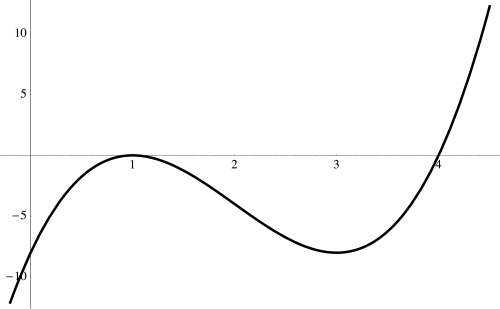  

Now let’s start looking at the behavior near the roots of this polynomial.

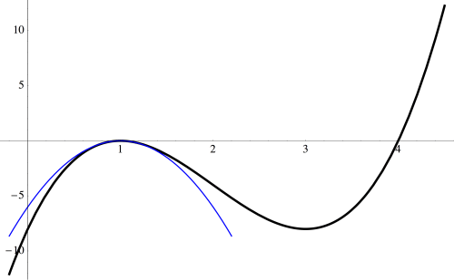
Near the graph of the cubic looks like a parabola — and that may not be so surprising given that the factor occurs quadratically.

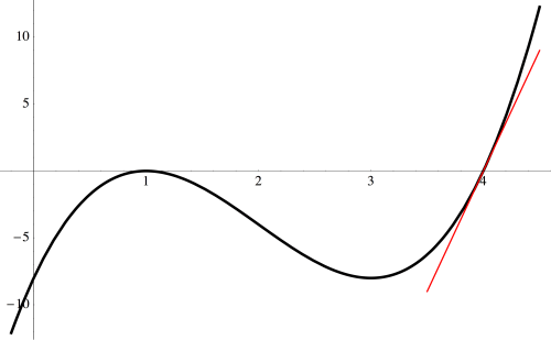
And near the graph passes through the x-axis like a line — and we see a linear factor of in our polynomial.

But which parabola, and which line?  It’s actually pretty easy to figure out.  Here is an annotated slide which illustrates the idea.

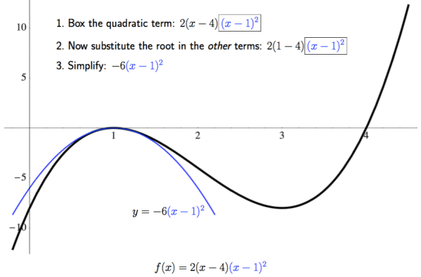
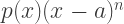
All you need to do is set aside the quadratic factor of and substitute the root, in the remaining terms of the polynomial, then simplify.  In this example, we see that the cubic behaves like the parabola near the root Note the scales on the axes; if they were the same, the parabola would have appeared much narrower.

We perform a similar calculation at the root

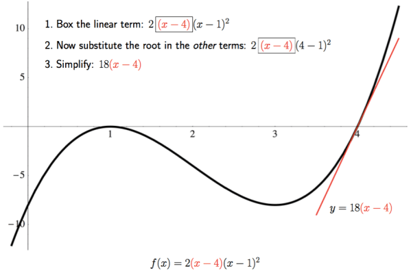
Just isolate the linear factor substitute in the remaining terms of the polynomial, and then simplify.  Thus, the line best describes the behavior of the graph of the polynomial as it passes through the x-axis.  Again, note the scale on the axes.

We can actually use this idea to help us sketch graphs of polynomials when they’re in factored form.  Consider the polynomial  Begin by sketching the three approximations near the roots of the polynomial.  This slide also shows the calculation for the cubic approximation.

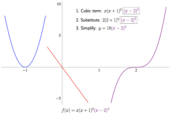
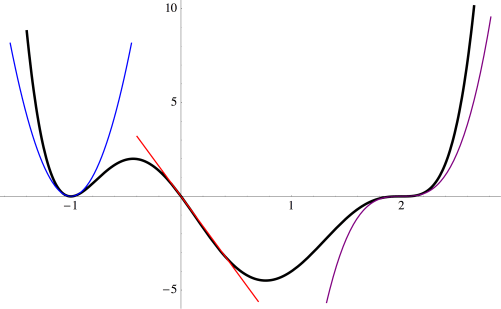
Now you can begin sketching the graph, starting from the left, being careful to closely follow the parabola as you bounce off the x-axis at

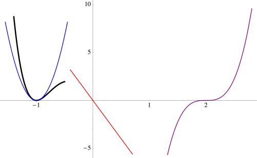
Continue, following the red line as you pass through the origin, and then the cubic as you pass through  Of course you’d need to plot a few points to know just where to start and end; this just shows how you would use the approximations near the roots to help you sketch a graph of a polynomial.

Why does this work?  It is not difficult to see, but here we need a little calculus.  Let’s look, in general, at the behavior of near the root  Given what we’ve just been observing, we’d guess that the best approximation near would just be

Just what does “best approximation” mean?  One way to think about approximating, calculuswise, is matching derivatives — just think of Maclaurin or Taylor series.  My claim is that the first derivatives of and match at

First, observe that the first derivatives of both of these functions at  must be 0.  This is because will always be a factor — since at most derivatives are taken, there is no way for the term to completely “disappear.”

But what happens when the th derivative is taken?  Clearly, the th derivative of at is just  What about the th derivative of ?

Thinking about the product rule in general, we see that the form of the th derivative must be When a derivative of is taken, that means one factor of survives.

So when we take we also get  This makes the th derivatives match as well.  And since the first derivatives of and match, we see that is the best th degree approximation near the root

I might call this observation the geometry of polynomials. Well, perhaps not the entire geometry of polynomials….  But I find that any time algebra can be illustrated graphically, students’ understanding gets just a little deeper.

Those who have been reading my blog for a while will be unsurprised at my geometrical approach to algebra (or my geometrical approach to anything, for that matter).  Of course a lot of algebra was invented just to describe geometry — take the Cartesian coordinate plane, for instance.  So it’s time for algebra to reclaim its geometrical heritage.  I shall continue to be part of this important endeavor, for however long it takes….