Time for the sequel to last week’s post! Last week, I talked about a major change in my career — moving from the classroom to full-time consulting. This week, I’ll talk more about the mental/psychological aspects of the change.
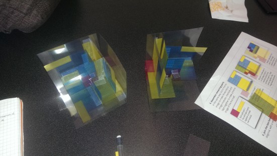
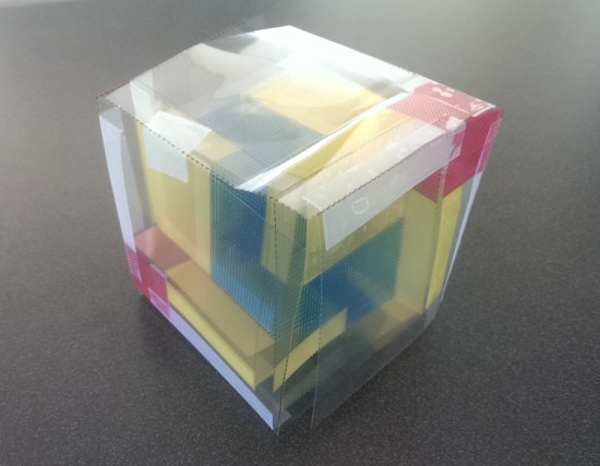
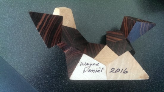
But first, I want to give a brief recap of our ninth Bay Area Mathematical Art Seminar. Because of my move — and lack of affiliation with a university — we met at a coffee shop in my new neighborhood at 3:00ish yesterday for show-and-tell and an informal discussion. One participant, Stan, brought a selection of puzzles from his extensive collection, which kept many of us occupied for some time. Of course we never have a shortage of things to talk about.
We then moved on, as usual, to dinner. It turns out that there is a fantastic Nepalese restaurant in Bernal Heights. We would typically find a Thai or Indian place near USF for dinner, and this Nepalese place was close to Indian in flavor — but better than any of the places we’d been to before.
I think we’ll be back again. So far, five from our group have offered to host a seminar on occasion. This means that if several of us host just one or twice a year, we can keep the group going. We are all very excited by this! One of my biggest worries was that finding a venue would be a big hurdle in keeping the seminars going, but we’ve already got volunteers for July and August. So full steam ahead!
This informal meeting didn’t warrant an entire blog post, but I wanted to make sure it was in the archives….
Back to the career change. The biggest issue was deciding whether or not to leave the brick-and-mortar academic environment. I will admit that I was pretty selective in terms of schools I applied to — since I had a backup plan, I had to think each time: would I prefer teaching in (insert location), or staying with my friends in Florida? I had lived in the middle of nowhere before — my first full-time teaching position was in west central Illinois. Can you name even one city in west central Illinois? I thought not….
I had actually done the Florida thing about four years ago while I was transitioning from Princeton to San Francisco — I spent six months there doing some online work and looking for jobs. So I knew it would be fine.
And then the consulting gig came into play. Totally unexpected. The process for bringing in consultants is way simpler than the process for bringing in new faculty members, which is why it took only about a month before I signed a contract. Keep in mind that I did this before knowing for certain whether or not the academic positions I applied for would amount to anything.
As you know, they didn’t. So was I willing to give a consulting career a chance? It was a lot riskier than an academic job. I have to admit that right now, things look pretty stable. But I’ve done some consulting before, and it can dry up all of a sudden. For example, I was consulting for a firm whose major client was considering dropping their account, and all resources went to making sure that client stayed on. I was expendable. It happens.
What about benefits? Oh, there are none…. No health insurance, no contributions to my retirement account. When teaching at USF, I applied for and was granted in excess of $15,000 for conference travel. In the summer of 2016, as an example, I was awarded $5000 for travel to two conferences in Europe. This perk would go away.
Further, could I handle working from home? As a professor, I was used to a lot of interaction with students and faculty on a regular basis. Now I’d be on my own during the day, every day. I talked a lot with friends Cory and Sandy about this particular issue.
You see, it’s different when you’re your own boss. I can tell you, since I’ve had an entire week’s experience at it…. When I was still teaching, every time I worked on one of my lectures for the online course and finished it, I’d think, “Hey, I’m getting ahead of the game! This’ll make my summer a little bit easier.” But when I woke up last Monday morning, all I could think was, “Oh, I am soooo far behind.”
Thankfully, I had a good long chat with my dear friend Cory, after which I sat down and made a brief — tentative — schedule of my entire summer. Then I felt much better, though there is still a big unknown: I haven’t produced a video yet (I’ll tackle my first one tomorrow!), so it is difficult to estimate how long that process will take. Though presumably it will take less time the more of them I make.
And working at home all the time? I’ve already had two “play dates” last week. Friends Nick and Stacy came over on two separate days, and we just worked on our own things together at my place. Yes, we chatted now and then, and I would occasionally answer some mathematical questions. But otherwise, we focused pretty well on our own work. I really enjoy working this way. It helps to have someone there, since you’re less likely to be distracted doing something useless online….
Also, I’m trying to find other activities which get me out interacting with other people. For example, I started going to the Gay Men’s Buddhist Fellowship on Sunday mornings again — I had done so for a few weeks about a year ago, but stopped once the academic year ramped up. But now, I’m making more of an effort.
Yes, it’s exciting, but no, it’s not glamorous. There’s potential to make more money than I did teaching, but there’s also the risk and added stress of being your own boss. The jury is still out.
One thing I am insistent upon is that I can do all my work remotely. I’ve already planned a trip to England and Serbia in October. And since the couple who owns the place I’m renting needs the apartment in January and February for family, I’ll be spending those months in Florida. It’s nice to have the flexibility to do that.
So let the adventure begin! I’ll probably continue this thread and let you know how things progress — maybe every three months or so. And if you’ve got any tips for working from home that you’d like to share, please comment! Until next time….
 and
and  then
then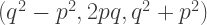
 for example, using this parameterization. Of course
  is just three times the triple
  therefore, if you can generate all primitive Pythagorean Triples, you can take multiples of them to generate all Pythagorean Triples.
 has side lengths which are in arithmetic progression. What other Pythagorean Triples have this property?
 where
where  is the smallest integer in the arithmetic progression and
  is the common difference. Since the triangle is a right triangle, we must have


 or
or  We did assume that
  so we eliminate the solution
  Note that this would generate the triple
  and in fact
 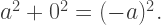 But one side length is zero and another is negative, so no triangle is possible with these side lengths.
 ? Here, we get
 of the primitive Pythagorean Triple
 right triangle.
 triangle, the area and perimeter were both
  A coincidence? Were there other triangles with this property?
 is necessary since the two-variable version generates all primitive Pythagorean Triples, but not necessarily all Pythagorean Triples.

 results in
 and the other two factors must be
 then
then  so that
  Substituting back into the parameterization, we obtain the Pythagorean Triple
  which is the triple
 then
then  so that
  This generates a new Pythagorean Triple,
 then
then  and
and  so that the Pythagorean Triple
  is generated. Of course this is just a duplicate of the first solution.
 and that their perimeters are equal. Prove that the triangles are congruent.
 is called the carrying capacity of the environment.
 is very small,
  and so the population growth is almost exponential. But when
  gets very close to
  then
then  and so population growth slows down. And of course when
  growth stops — hence calling
 and
and 


 and
and  to write
 and
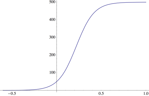
and  we need to scale by a factor of
  so that the asymptotes of the logistic curve are
 and
and 
 We can accomplish this be replacing
  with
with 
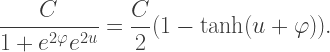


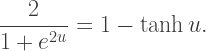
 is an odd function, becomes
 might be suggested, but how would we relate this to the exponential function?
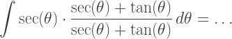
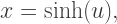
 using the hyperbolic trigonometric substitution
  Today, we’ll look at this substitution in more depth.
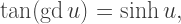
 and
and  is described by the gudermannian function, defined by
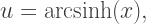
 so that this relationship is in fact invertible.
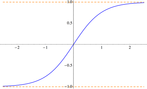
 to obtain the quadratic

 then
then  must be an increasing function of
  It is not difficult to see that we must choose “plus,” so that
  and consequently
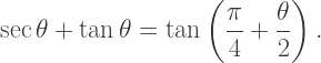
 by
by  in order to form an isosceles triangle. Thus,
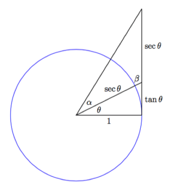
 observe that
  is supplementary to both
  and
and  so that

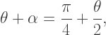

 giving
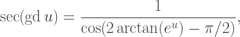


 giving
 Again using the usual circular trigonometric identities, we can show that
 and
and 
 is the inverse of the gudermannian function, then


 so that
 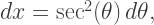 and the integral transforms to

 so that
  and
and 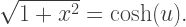 Note well that taking the positive square root is always correct, since
  is always positive!

 and
and
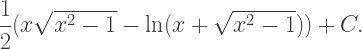
 and so our integral finally becomes
 What this means is — no need to ever integrate
 and
and  which involve integration by parts. Simply put, it is not a good use of time. I think it is far better to introduce students to hyperbolic trigonometric substitution.
 and transform the integral into
 We get
  and
and  (here, a negative square root may be necessary).

 which may be found using the same technique we used last week for


 and
and  may be computed by using the substitutions
  and
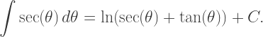
and  respectively. It bears repeating: no more integrals involving powers of tangents and secants!
 work above? For the same reason
  works: we can simplify
  using one of the following two identities:
 is playing the role of
  and
and  What does that suggest? Try using the substitution
  !
! we have
 — just look at the above identities and compare. We remark that if
  then as a result of the asymptotic behavior, the substitution
  and between the graphs of
  In this case, the signs are always correct —


 so there is no need to put the argument of the logarithm in absolute values.
 or
or 
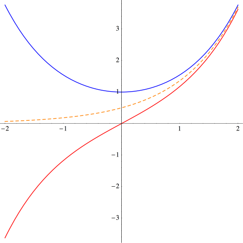
 is shown in blue, and the graph of
  is shown in red. The dashed orange graph is
  which is easily seen to be asymptotic to both graphs.
 is an even function, just like
 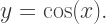 Similarly,

 lies on a unit hyperbola, much like
  lies on a unit circle.
 Recall that given any function
  we may define
 respectively.


 to
to  to
to  sometimes changes of sign are necessary.

 and
and  Gone are the days of remembering signs when differentiating and integrating trigonometric functions! This is one feature of hyperbolic trigonometric functions which students always appreciate….

 for
for  Begin with the definition:


 is always negative, so that we must choose the positive sign. Thus,
 or
or  These get students working with the definitions and thinking about asymptotic behavior.
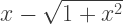
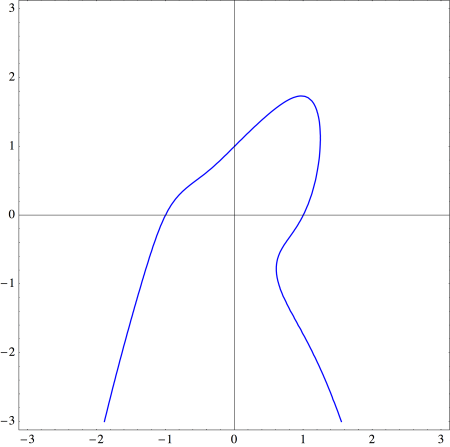
 where it crosses the x-axis at
  we simply retain the
  term and substitute the root
  into the other terms, getting

 (the U-shaped piece, since the sideways U-shaped piece involves writing
  as a function of
  ) is
) is  as shown below.
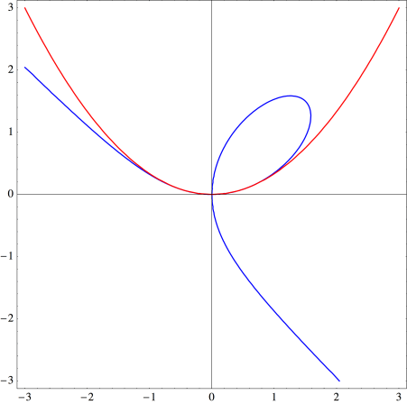

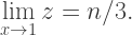
 and so rewrite the equation for the Folium of Descartes by using the substitution
  which results in
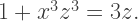
 we have
  giving us a good quadratic approximation at the origin.
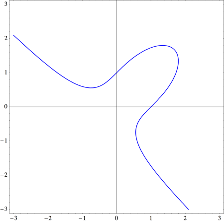
 looking at the curve

 with
with 
 we have
 Thus, in our case with
  we see that
  is a good approximation to the curve near the origin. The graph below shows just how good an approximation it is.
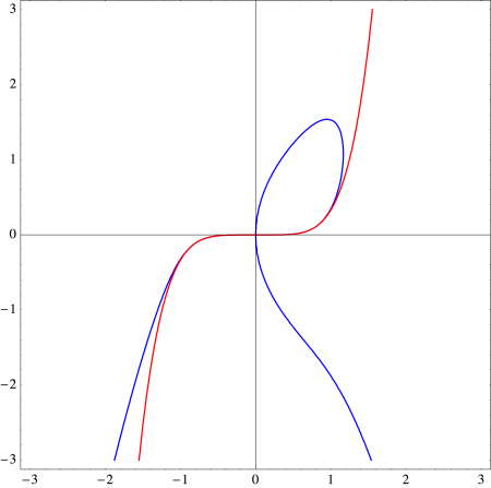

 which results in
 here. But if we move the
  to the other side and factor, we get
 to obtain
 And sure enough, the line
  does the trick:
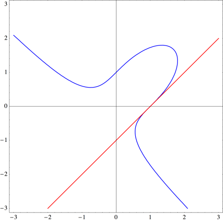


 This results in
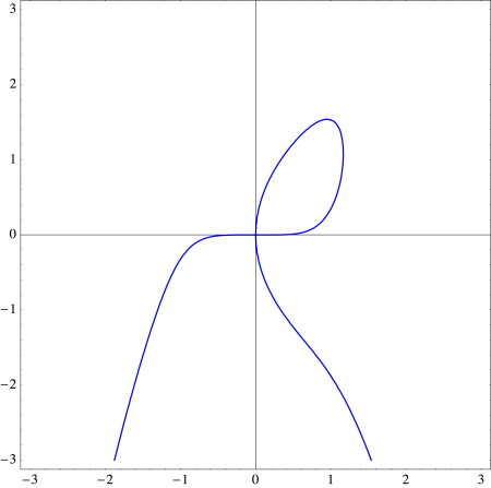
 is even, since there is always a root at
  in this case. Here, we make the substitution
  move the
  resulting in
 is a factor of
  so we have

 as well! This is a curious coincidence, for which I have no nice geometrical explanation. The case when
  is illustrated below.
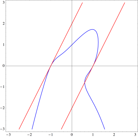


 Look carefully, and you’ll see that no single edge in any of these dissections exactly matches any other. For these decompositions, Scott has proved they are minimal — so, for example, there is no motley dissection of one pentagon to ten or fewer. The proofs are not exactly elegant, but they serve their purpose. He also mentioned that he credits Donald Knuth with the term motley dissection, who used the term in a phone conversation not all that long ago.