Creativity in Mathematics

Beguiling Games III: Splotch!

In this installment of Beguiling Games, we’ll learn how to play Splotch!

Day119Splotch1

But first, I’ll start off by giving you the solution to the last puzzle I presented in the last installment. The statement of the puzzle is too long to repeat, so you can refresh your memory at Beguiling Games II.

First, it is important to note that Lucas’s statement actually provides no information! Suppose Ophelia’s card was Truthteller. Then she would have told the truth in Round 1, passed her card to Lucas, and he would truthfully have stated that she told the truth in Round 1.

But what if Ophelia’s card was Liar? Then her statement “I am a Truthteller” in Round 1 would in fact have been a lie. Now she passes her card to Lucas. He lies and says she told the truth in Round 1! What this means is Lucas could have made his statement in Round 2 regardless of what card Ophelia passed him.

Note that the same logic applies to Mordecai’s statement. He could have said “Lucas also told the truth in the first round” regardless of whether Lucas passed him a Truthteller or a Liar card.

Now let’s examine Nancy’s statement in some detail. She said that there is at least one liar at the table. Could she have lied?

Well, if the fact that the there is at least one liar at the table is false, that means everyone is a Truthteller. But there is no way Nancy could have known this, since the only two cards she saw were hers and the card passed to her by Mordecai.

That means Nancy must have told the truth in Round 2, and Mordecai must have passed her a Truthteller card. But in order for her to have sufficient information to say there is at least one Liar at the table, she must have been holding a Liar card in Round 1.

Now this information could be deduced by anyone at the table. In other words, anyone would know that Nancy held a Liar card in Round 1, and Mordecai held a Truthteller card. That leaves Lucas’s and Ophelia’s cards in Round 1.

The only person who could know both these cards would be Lucas — he knew his own card in Round 1, and he knew Ophelia’s card because she passed it to him in Round 2. So he had enough information to declare after Nancy’s statement.

It is important to point out that there is no way to know what Lucas’s and Ophelia’s cards actually were. All we need to know is that Lucas knew what both of them were.

Did you figure it out? It takes a little bit of reasoning, but all the facts were there.

Now as I mentioned in the last installment, this time I’d give you a geometrical two-player game to work out. I call it Splotch!

In the game of Splotch!, players alternate coloring in squares on a 4 x 4 grid. The goal is to create a target shape, called a splotch. A player wins when he or she colors in a square which completes a splotch, and then announces the win.

So if a player completes a splotch but doesn’t notice it and doesn’t announce the win, then play continues until someone completes another splotch. You can only call Splotch! on your turn, so you cannot win by calling it if your opponent fails to. It is also important to remember that the square you color in on your turn must be part of a splotch you announce.

In the version of Splotch! I’m sharing with you this week, the target splotch is:

Day119Splotch1

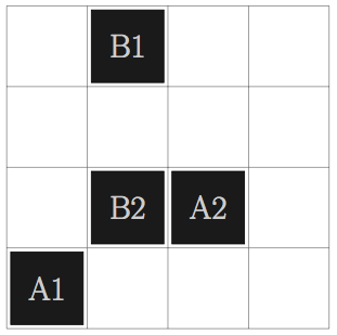
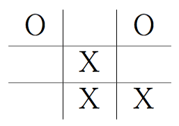
Just so you know how it works, let’s look at a sample game, shown below.

Day119Splotch2

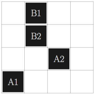
There are two players, A and B. A goes first, and plays in the lower left corner (labelled with A1). B colors in a square in the top row (B1). Then A’s second move is in the second row. B wins on the next play by completing — and announcing! — a splotch. The splotch may be rotated (as in this example), reflected, or even both! So you’ve got to watch carefully.

Now admittedly, A was not a very clever player in this round of Splotch! In fact, B could also have won by playing as follows:

Day119Splotch3

But here is the question: In this version of Splotch!, which player can force a win every time? Remember: you must be able to provide a response to every move by your opponent! I’ll reveal which player can force a win in my next installment of Beguiling Games, and I’ll share my particular strategy for winning.

One final remark — a bit of a tangent, but related to puzzles and games. If you’ve been following my blog for a long while, you might remember my (fiendishly diabolical) number searches. (These were posted well over a year ago.)

Day031Fig1

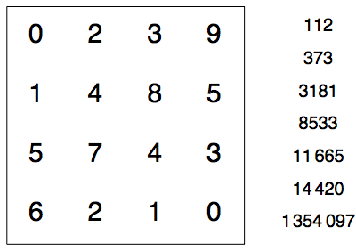
Here, the numbers in the right are in base 10, but you have to convert them to another base to find them in the grid! You can read more about these puzzles here and here.

I submitted these puzzles to MAA Focus, the newsmagazine of the Mathematical Association of America. I am happy to report that they will be featured on the Puzzle Page in the December 2017/January 2018 issue!

Now I will admit that this doesn’t exactly make me famous, given the number of people who subscribe to MAA Focus. But I composed these puzzles specifically for my blog — so if I hadn’t decided to write a blog, these puzzles might never have been created. Perhaps another reason to write a blog!

Stay tuned for the next round of Beguiling Games, where you’ll learn (if you didn’t already figure it out for yourself) who has a winning strategy in the game of Splotch!

Geometrical Dissections III: Octagons and Dodecagons

It has been quite a while since I’ve written about geometrical dissections. For a brief refresher, you might want to look at my first post on dissections.

But recently my interest has been rekindled — to the point that I started writing a paper a few weeks ago! I often like to share mathematics I’m working on as it’s happening to give you some idea of the process of doing mathematics. The paper has quite a bit more mathematics in it than I’ll include in this post, but I’ll try to give you the gist of what’s involved.

Recall (again, see my first post for a more thorough discussion) that I’m interested in finding dissections that you can draw on graph paper — I find these more enjoyable as well as being accessible to a wider audience. So all the dissections I’ll talk about will be based on a grid.

The first example is a dissection of two octagons to one, such as shown below.

Day118Dissection2

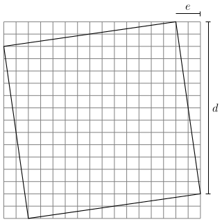
In other words, you can take the pieces from the two smaller octagons, move them around, and build the larger octagon. If you look carefully, you’ll notice that the larger octagon is rotated 45° relative to the smaller octagons. Geometrically, this is because to get an octagon twice the area of a given octagon, you scale the side lengths by $\sqrt2.$ Imagine a square — a square with side length $S$ has area $S^2,$ while a square with side length $\sqrt2S$ has area $(\sqrt2S)^2=2S^2$ — which is double the area.

Now think of a segment of unit length. To get a segment of length $\sqrt2,$ you need to take a diagonal of a unit square, which rotates the segment by 45° as well as scales it by a factor of $\sqrt2.$ This is why the larger octagon is rotated with respect to the smaller ones.

But what makes this dissection interesting is that there is an infinite family of very similar dissections. By slightly varying the parameters, you get a dissection which looks like this:

Day118Dissection3

Here, you can clearly see the 45° rotation of the larger octagon. I always enjoy finding infinite families of dissections — it is very satisfying to discover that once you’ve found one dissection, you get infinitely many more for free!

The proof that this always works (which I will omit here!) involves using a geometrical argument — using arbitrary parameters — to show that the green triangles always have to be right isosceles triangles. This is the essential feature of the dissection which makes it “work” all the time.

The second example I’m including in the paper is a dissection on a triangular grid, like the one below.

Day118Dissection4

Note that the figure on the left is an irregular dodecagon; that is, it has twelve sides. Recall that the interior angles of a regular dodecagon have measure 150° — but so do the angles of this irregular dodecagon as it is drawn on a triangular grid.

If you look carefully, you’ll see how the sides in the pieces of the dissection on the right match up with sides of the same length from the other pieces. Also, looking at the dissection on the right, you’ll see that around all the interior vertices, there are two angles with measure 150° and one with measure 60°, adding up to 360° — as we would expect if the pieces fit exactly together.

And — as you might have guessed from the first example — this is also one of an infinite family of dissections. As long as the sides of the irregular dodecagon alternate and the vertices stay on the triangular lattice, there is a dissection to a rhombus. Below is another example, and there are infinitely many more….

Day118Dissection5

My third and final example involves irregular dodecagons, but this time on a square grid. And while I found the previous two dissections several years ago, I found this example just last week! What inspired me was one of my favorite dissections — from an irregular dodecagon to a square — also found many years ago.

Day118Dissection1

In the spirit of the first two examples, I asked myself if this dissection could be one of an infinite family. The difficulty here was that there were three parameters determining an irregular dodecagon, as shown below.

Day118Dodecagon

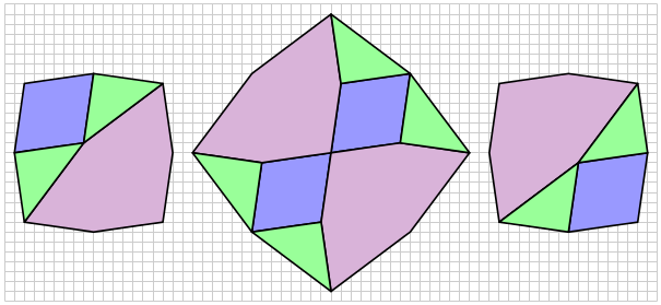
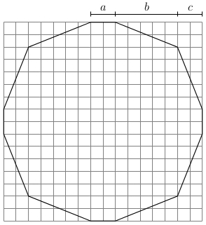
We do need $b>c$ so that the dodecagon is convex and actually has 12 sides; if $b=c,$ four pairs of sides are in perfect alignment and the figure becomes an octagon.

There is an additional constraint, however, which complicates things a bit. The area of this dodecagon must also be the area of some tilted square with vertices on the grid, as illustrated below. Note that the area of this square is just $d^2+e^2.$

Day118Square

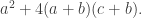
It is not a difficult geometry exercise to show that the area of the dodecagon is $a^2+4(a+b)(c+b).$ So in order to create a dissection, we must find a solution to the equation

$a^2+4(a+b)(c+b)=d^2+e^2.$

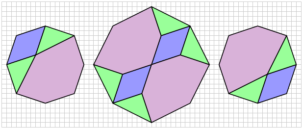
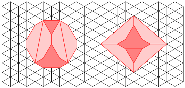
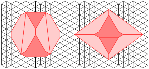
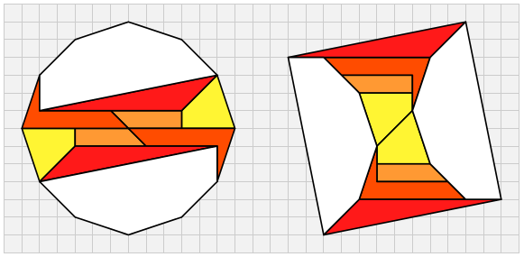
Again, here is not the place to go into details. But it is possible to find an infinite family of solutions when $a=e.$ You get a dissection which looks like this:

Day118Dissection6

I was particularly pleased to have found this eight-piece dissection since most of my attempts until this point had ten pieces or more. And to give you a sense of this family of dissections, here is an example with different parameters within this family.

Day118Dissection7

You can definitely see the resemblance, but it is also clear that the dodecagon and square are not the same shape as those in the previous dissection.

So these are the three families of geometrical dissections I’ll be including in my paper. I hope these examples might inspire you to pick up a pencil and graph paper and try to find some infinite families of your own!

On Coding XII: Python

It has been some time since I wrote an installment of On Coding. It’s time to address one of my more recent programming adventures: Python. I started learning Python about two-and-a-half years ago when I began teaching at the University of San Francisco.

One of my colleagues introduced me to the Sage environment (now going by “CoCalc”) as a place to do Mathematica-like calculations, albeit at a smaller scale. Four features were worthy of note to me: 1) you could do graphics; 2) you could write code (in Python); 3) you could run the environment in your browser without downloading anything; and 4) it was open source.

For me, this was (at the time) the perfect environment to develop tools for creating digital art which I could freely share. Yes, I had thousands of lines of Mathematica code, but Mathematica is fairly expensive. I wanted an environment which would be easily accessible to students (and my blog followers!), and Sage fit the bill.

So that’s why I started learning Python — it was the language I needed to learn in order to use Sage.

For me, two things were a challenge. The first was how heavily typed Python is. In Mathematica, the essential data structure is a list, just like in LISP. For example,

{1, 2, 3}

is a list. But that list may also represent a vector in three-dimensional space — even though it would look exactly the same. It may also represent a set of numbers, so you could calculate

Intersection[{1, 2, 3}, {3, 4, 5}].

In Python you can create a list, tuple, or set, as follows:

list([1, 2, 3]), tuple([1, 2, 3]), set([1, 2, 3]).

And in Python, these are three different objects, none equal to any other. I don’t necessarily want to start a discussion of typed vs. untyped languages, but when you’re so used to using an untyped language, like Mathematica, you are constantly wondering if the argument to some random Python function is a list, tuple, or….

Second, Python has a “return” statement. In languages like LISP and Mathematica, the value of the last statement executed is automatically returned. In Python, you have to specify that you want a value returned by using a return statement. I forget this all the time.

And while not a huge obstacle, it does take a little while to get used to integer division. In Python, 3/4 = 0, since when you divide integers, the value of the fraction is the quotient when considered as integer division. But 3/4. = 0.75, since adding the decimal point after the 4 indicates the number is a floating point number, and so floating-point arithmetic is performed.

Of course, if you’ve been reading recent posts, you know I’ve moved from Sage entirely to Processing in my Mathematics and Digital Art course. You can read more about that decision here — but one key feature of Processing is that there’s a Python mode, so I was able to take work already done in Sage and adapt it for Processing.

It turns out that this was not as easy as I had hoped. The essential difficulty is that in Sage, the bounding box of your image is computed for you, and your image is appropriately scaled and displayed on the screen. In Processing, you’ve got to do that on your own, as well as work in a space where x– and y-coordinates are in units of pixels, which is definitely not how I am used to thinking about geometry.

I am finding out, however — much to my delight and surprise — that there are quite a few functional programming aspects built into Python. I suspect there are many more than I’m familiar with, but I’m learning them a little at a time.

For example, I am very fond of using maps and function application in Mathematica to do some calculations efficiently. Rather than use a loop to, say, add the squares of the numbers 1– 10, in Mathematica, you would say

Plus @@ (#^2& /@ Range[10])

The “#^2&” is a pure function, and the “/@” applies the function to the numbers 1–10 and puts them in a list. Then the function “Plus” is applied, which adds the numbers together.

There is a similar construct in Python. The same sum of 385 can be computed by using

sum([(n + 1)**2 for n in range(10)])

OK, this looks a little different, but it’s just the syntax. Rather than the “#” character for the variable in the pure function, you provide the variable name. The “for” here is called list comprehension in Python, though it is just a map. Of course you need “(n + 1),” since Python always starts at 0, so that “range(10)” actually refers to the numbers 0–9. And the “sum” function can take a list of numbers as well. But from a conceptual level, the same thing is going on.

The inherent “return” in any Mathematica function does find its way into Python as well. Let’s take a look at a simple example: we’ll write a function which computes the maximum of two numbers.

Now you’d probably think to write:

Day117python1

This is the usual way of defining “max.” But there’s another way do to this in Python.

If you ask Python to

print 3 > 2,

you’ll see “True.” But you can also tell Python to

print (3 > 2) + 7

and get “8.” What’s going on here is that depending on the context, “3 > 2” can take on the value “True” or “1.” Likewise, “3 < 2” can take on either the value “False” or the value “0.”

This allows you to completely sidestep making Boolean checks. Consider the following definition.

Day117python2

This also works! If in fact a >= b, you return the value 1 * a + 0 * b, which gives you a — the maximum value when a >= b. And when a < b, you return b. Note that when a = b, both are the maximum, so we could just as well have written

Day117python3

I think this is a neat feature of Python, which does not have a direct analogue in Mathematica. I am hoping to learn many other intriguing features like this as I dive deeper into Python.

Python is my newest language, and I have yet to become “fluent.” I still sometimes ask the internet how to do simple things which would be at my fingertips in Mathematica. But I do love learning new languages! Maybe in a year or so I’ll update my On Coding entry on Python with a flurry of new and interesting things I’ve learned….

Bay Area Mathematical Artists, II

Yesterday was the second meeting of the Bay Area Mathematical Artists! We had a somewhat different group — some who came last time were unable to make it, but there were some new faces among the enthusiasts as well. Fourteen showed up for the afternoon, and two others joined us for dinner afterwards.

After the last meeting, I received a few emails offering suggestions about different ways to organize the gatherings. One suggestion was to have a social period for the first part of the meeting, where participants could meet those they didn’t already know, or perhaps bring artistic items for show-and-tell.

This seemed like a good idea, since in addition to letting participants get to know each other or just catch up on the previous month, it gave them a 30-minute buffer to arrive on campus. It turns out this part of the afternoon went very well, with just about everyone arriving by 3:30. Dan Bach was giving away old copies of mathematics journals he had collected over the years, while Colin Liotta was giving away laser-etched wooden pendants.

The only scheduled talk of the afternoon was given by Roger Antonsen, entitled Mathematical explorations and visualizations.

Day116Roger

Roger talked about several of his extensive library of Processing animations. He takes his inspiration from many different places – but his Processing mantra is sometimes “make it move.” He takes an image which fascinates him, recreates it as best as he can, and then varies different parameters to make the image move.

Some of his most intriguing examples involved optical illusions, and are based on the work of Pinna; see his web page on Art to see some examples.

He also emphasized the need to create balance in his work – when you parameterize features of an image, you need to decide the range the parameter takes. Too much motion, and the animation looks too distorted, but too little, and the animation is too static. Of course the need to create balance in artwork is not restricted to creating animations, but it is constantly in Roger’s mind as he creates.

After Roger’s talk, we moved on to a discussion about the nature of mathematical and digital art. There are other similar terms in use, such as algorithmic art and generative art. Typically, generative art is described as art generated by some autonomous system. This means that algorithmic art — that is, art created by use of a computer program — is a subset of generative art. But what do all these terms mean to us, individually, as artists?

I had originally thought to break into smaller groups at first, but the group wanted to have just one, larger discussion.

There were many and varied opinions expressed — from commentary about the art community as a whole, to those who thought the question “What is mathematical art?” is nonsensical to ask because there is really no answer, and it doesn’t impact the creative process at all.

Two points I made relate to my teaching Mathematics and Digital Art. First, every time you settle on the value for a parameter in some work you’re doing, you are making an aesthetic choice. You can tweak all you like, but then all of a sudden you just say to yourself, “OK, that’s it!” Of course there are times you just stop because you can’t find precisely what you want and just need to move on, but I think you get the gist of what I’m saying. You’re making artistic choices all the time.

And second, I have students write short narratives about their work, describing the parameter choices they make. I want to them to think about when a digital image becomes a piece of digital art. Of course (as alluded to above) there really is no definitive answer to this question, but for students just beginning to dive into the world of digital and mathematical art, it is a useful question to consider.

This took us right to our designated ending time, 5:00. One of the participants suggested a Thai place nearby, and so eleven of us made the short trek just north of campus. It was actually quite good, according to all accounts. And as I mentioned earlier, two participants who couldn’t make it earlier in the day joined us at the restaurant. The discussions were lively, covering a broad range of mathematics, art, and other topics as well.

So again, a good time was had by all! To round out today’s post, I’d like to say a few words about the new Digital Art Club I’m advising at the University of San Francisco. It seems each week, one or two more students become interested, mostly by word of mouth. There are new faces all the time!

It turns out this is a great opportunity for mathematics or science majors to learn about digital art. The Mathematics and Digital Art course I’m teaching is not at a high enough level to count towards a mathematics major, and many students in the sciences (like computer science or physics) have required mathematics courses, also at a higher level.

We’re focusing on learning Processing at the moment, since not only are students very interested in learning the software, but I have written quite a bit about Processing on my blog. So I can easily get students started by pointing them to an appropriate post.

Not only that, we’ve got a few students willing to take leadership positions and secure status as an officially recognized student club. This means there are funds available for field trips and other activities. We’re hoping to make a trip to the Pace Gallery in Palo Alto. I’ll occasionally update on our progress in future posts. Stay tuned!

Mathematics and Digital Art: Update 2 (Fall 2017)

We’ve just completed Week 8 of the Fall semester, so it’s time for the next update on my Mathematics and Digital Art class! As I had mentioned before, the major difference this semester was starting with Processing right from the beginning of the semester.

It turns out this is making a really big difference in the way the class is progressing. The first two times I taught the course, I had students work in the Sage environment for the first half of the semester. The second half of the semester was devoted to Processing and student projects.

Because students only started to learn Processing at the same time they were diving into their projects, they were not able to start off with a Processing-based project. As it happened, a few students actually incorporated Processing into their final projects as the second half of the semester progressed, but this was the exception, not the rule.

But last week, we already started making movies in Processing! Starting simply, of course, with the dot changing colors.

This was a bit easier to present this time around, since we already had a discussion of user space vs. screen space earlier in the semester. So this time, I could really focus on linear interpolation — the key mathematical concept behind making animations.

Next week will be a Processing-intense week. I’ll delay some topics — like geometric series — to a little later in the course so we can get more Processing in right now. The reason? I really think many students will involve Processing in their final projects in a significant way. I want to make sure they have enough exposure to feel confident about going in that direction for their final projects. I’ll let you know what happens in this regard in my next update of Mathematics and Digital Art.

Now for some examples of student work! For the assignment on iterated function systems, students had three different images to submit. The first was a Sierpinski triangle — I asked students to create an image simultaneously as close to and as far away from a Sierpinski triangle as possible. The idea was that a viewer should recognize the image as being based on a Sierpinksi triangle, but perhaps only after staring at it for thirty seconds or so.

This is Sepid’s take on the assignment. On many of her pieces, she experimented with different ways to crop the final image. This has a significant effect on the image’s final appearance.

This is Cissy’s submission for the Sierpinski triangle. In this piece (and the others submitted for this assignment), Cissy remarked that she really enjoyed experimenting with color. I commented that I thought color choices were among the most difficult decisions to make as far as elements of a work of digital art are concerned.

The second piece was to involve only two affine transformations. This is often a challenge for students, but there really is an enormous variety of images that may be created using just two transformations. In addition, one of the transformations needed to involve a rotation by a non-trivial angle (that is, not a multiple of 45°), and students needed to submit a picture of their calculations as well.

One student was trying to create an image that looked like an animal footprint. She remarked that she did consider a different color palette, but in the end, preferred to go with monochromaticity.

Interestingly, Terry also used a simple color palette. She remarked that it was challenge to use just two transformations — and because of this minimalist requirement, decided to go with a minimalist color palette. In addition, her resulting fractal reminded her of birds, so she set the fractal against a white moon and gray sky.

Day115Terry2

For the third submission, there were no constraints whatsoever — in fact, I encouraged students to be as creative as possible. There was a very wide range of submissions. One student was fairly minimalistic, using a highly contrasting color palette.

Day115A

Jack’s piece was also fairly minimalistic. I should remark that we took part of a lab one day for students to do some online peer commenting; Jack (and others as well) remarked that he used the advice of another student to improve an earlier draft of his piece. In particular, he adjusted the stroke weight to increase the intensity of the colors.

Tera based her work on the Sierpinski triangle, but also included reflections of each of the three smaller components of her version of the Sierpinski triangle. She remarked that the final image reminded her of a snowflake, or perhaps a Christmas sweater.

Alex’s inspiration came from The Great Wave off Kanagawa, by Katsushika Hokusai.

First, he created the fractal image, experimenting with various color combinations. When he was satisfied with his palette, he added the boat and the white circle to suggest a black moon. A rather interesting approach!

As you can see, I’ve got quite a creative class of students who are willing to experiment in many different ways. It’s interesting for me, since there is no way to predict what they’ll create next! I look forward to seeing what they create when they really dive deeply into Processing and begin making animations.

In the next update, I’ll report on how students involve Processing in their project proposals. In addition, they will have submitted their fractal movie projects by then, so there will undoubtedly be many interesting examples of student work to exhibit. Stay tuned!

Beguiling Games II: Nuh-Uh!

First, we’ll look at the game I left you with in the last installment of Beguiling Games. These were the rules of yet another variation of Tic-Tac-Toe: if during the game either play gets three-in-a-row, then X wins. If at the end, no one has three in a row, then O wins. Does X have a winning strategy? Does O? Why?

We’ll show that X has a winning strategy. As with usual Tic-Tac-Toe, X starts at the center. If O goes in any square which is not a corner, then X will win as a result of the winning strategy in Tic-Tac-Toe. So all that’s left to do is look at the case when O goes in a corner. Let’s suppose it’s the upper right corner.

Then X goes in the lower right corner. O must block, or else X will get three-in-a-row and win (since X wins if either player gets three-in-a-row). So now, the board looks like this:

Day114a

Take a moment to see if you can figure out X’s winning strategy. Do you see it? All X needs to do is place in the center of the bottom row.

Day114b

Look at the top row. Someone eventually has to place an X or O in this location. No matter which one, a three-in-a-row will be created, and X will win! So in this version of Tic-Tac-Toe, X has a winning strategy.

Today’s game will involve a different dynamic — cards and logic. But first, let me give a little bit of context. I have often used the book Problem Solving in Recreational Mathematics by Averbach and Chien when I’ve taught an introduction to proofs course. There are many interesting problems in this book, and the chapter on logic has several problems involving Truthtellers and Liars.

So you have to solve problems by figuring out who are the Truthtellers and who are the Liars. I like to use these problems to get students writing arguments in complete sentences since not only are they fun to work out, but they don’t involve notation. Using notation correctly is another issue entirely, and I prefer to deal with that later on in the course.

As before, there’s a story to go along with the game….

Lucas, Mordecai, Nancy, and Ophelia decided that enough was enough, and so ended their Saturday afternoon’s cramming for the National Spelling Bee. Wondering what they might do to pass the time, Lucas suggested, “Let’s play Nuh-Uh!” Everyone enthusiastically agreed.

And so a game of Nuh-Uh! — whose creators, incidentally claim that it is the only game on the market which “Tortures your Mind, Warps your Character, and Impoverishes your Soul — all at the Same Time!” — commenced.

So Lucas shuffled the deck of eight cards; four of the cards had the word Truthteller on them, and four had the word Liar. Dealing from the left, Lucas first dealt a card to Mordecai, then one to Nancy, one to Ophelia, and then finally one to himself. Cards are dealt face down so a player can only see his or her card.

Per the rules of Nuh-Uh!, Lucas, then Mordecai, Nancy, and finally Ophelia made the statement “I am a Truthteller.” Of course, such a statement was consistent with each player’s card, regardless of what was written on it. Thus ended the first round.

In subsequent rounds, each player passes his or her card to the player on the left, and makes a statement consistent with the new card. Thus, if Lucas passed Mordecai a card with Liar written on it, Mordecai would have to make a statement which is false. The statement a player makes is based on the knowledge of the cards he or she has seen, and any other information which may be deduced from the statements of the previous players.

The same player begins each round of making statements. So Lucas began each round in this game. Once the game is over, the deal passes to the left, so Mordecai would deal and begin each round with a statement.

After a player makes a statement, players may, beginning with the player on the left of the one who just spoke, “Declare” — that is, say what card each of the players held during the first round. The declaring player then looks at the cards held by the players to decide if he or she has won. If an error is made in declaring, the player drops out and play continues; otherwise the cards are turned over and the deal passes to the next player on the left.

So the players passed their cards to the left, and thus the second round of making statements began. Lucas started off with “Ophelia told the truth in the first round.” After a polite few seconds of pause to give someone a chance to declare, Mordecai said, “Lucas also told the truth in the first round.”

Another brief pause ensued before Nancy stated, “There is at least one liar at the table.” Note: there are four Truthteller and four Liar cards, so it is possible that all players were dealt a Truthteller card.

After Nancy made her statement, one of the players had enough information to declare and win the game. Which player declared?

Yes, there are enough clues to solve this! But a word of caution — the solution to the puzzle only involves answering the question, “Which player declared?” There may not be enough information to give a more complete answer….

Good luck! In the next installment of Beguiling Games, I’ll give the solution to this logic puzzle, and give a geometrical two-player game to analyze as well. Happy solving!

Creating Animated GIFs in Processing

Last week at our Digital Art Club meeting, I mentioned that I had started making a few animated gifs using Processing. Like this one.

GIF

(I’m not sure exactly why the circles look like they have such jagged edges — must have to do with the say WordPress uploads the gif. But it was my first animated gif, so I thought I’d include it anyway.)

And, of course, my students wanted to learn how to make them. A natural question. So I thought I’d devote today’s post to showing you how to create a rather simple animated gif.

sample

Certainly not very exciting, but I wanted to use an example where I can include all the code and explain how it works. For some truly amazing animated gifs, visit David Whyte’s Bees & Bombs page, or my friend Roger Antonsen’s Art page.

Here is the code that produces the moving circles.

gif3

I’ll assume you’ve done some work with Processing, so you understand the setup and draw functions, you know that background(0, 0, 0) sets the background color to black, etc.

The idea behind an animated gif which seems to be a continuous loop is to create a sequence of frames whose last frame is essentially the same as the first. That way, when the gif keeps repeating, it will seem as though the image is continually moving.

One way to do this is with the “mod” function — in other words, using modular arithmetic. Recall that taking 25 mod 4 means asking “What is the remainder after dividing 25 by 4?” So if you take a sequence of numbers, such as

1, 2, 3, 4, 5, 6, 7, 8, 9, 10, 11, 12, 13, 14, …

and take that sequence mod 4, you end up with

1, 2, 3, 0, 1, 2, 3, 0, 1, 2, 3, 0, 1, 2, ….

Do you see it already? Since my screen is 600 pixels wide, I take the x-coordinate of the centers of the circles mod 600 (that’s what the “% 600” means in Python). This makes the image wrap around horizontally — once you hit 600, you’re actually back at 0 again. In other words, once you go off the right edge of the screen, you re-enter the screen on the left.

That’s the easy part…. The geometry is a little trickier. The line

x = (75 + 150 * i + 2 * frameCount) % 600

requires a little more explanation.

First, I wanted the circles to be 100 pixels in diameter. This makes a total of 400 pixels for the width of the circles. Now since I wanted the image to wrap around, I needed 50 pixels between each circle. To begin with a centered image, that means I needed margins which are just 25 pixels. Think about it — since the image is wrapping around, I have to add the 25-pixel margin on the right to the 25-pixel margin on the left to get 50 pixels between the right and left circles.

So the center of the left circles are 75 pixels in from the left edge — 25 pixels for the margin plus 50 pixels for the radius. Since the circles are 100 pixels in diameter and there are 50 pixels between them, there are 150 pixels between the centers of the circles. That’s the “150 * i.” Recall that in for loops, the counters begin at 0, so the first circle has a center just 75 pixels in from the left.

Now here’s where the timing comes in. I chose 300 frames so that by showing approximately 30 frames per second (many standard frame-per-second rates are near 30 fps) the gif would cycle in about 10 seconds. But cycling means moving 600 pixels in the x direction — so the “2 * frameCount” will actually give me a movement of 600 pixels to the right after 300 frames. You’ve got to carefully calculate so your gif moves at just the speed you want it to.

To make displaying the colors easier, I put the R, G, and B values in lists. Of course there are many other ways to do this — using a series of if/else statements, etc.

One last comment: according to my online research, .png files are better for making animated gifs, while .tif files (as I’ve also used in many previous posts) are better for making movies. But .png files take longer to save, which is why your gif will look like it’s moving slowly when you use saveFrame, but will actually move faster once you make your gif.

So now we have our frames! What’s next? A few of my students mentioned using Giphy to make animated gifs, but I use GIMP. It is open source, and can be downloaded for free here. I’m a big fan of open source software, and I like that I can create gifs locally on my machine.

Once you’ve got GIMP open, select “Open as Layers…” from the File menu. Then go to the folder with all your frames, select them all (using Ctrl-A or Cmd-A or whatever does the trick on your computer), and then click “Open.” It may take a few minutes to open all the images, depending on how many you have.

Now all that’s left to do is export as an animated gif! In the File menu, select “Export As…”, and make sure your filename ends in “.gif”. Then click “Export.” A dialog box should open up — be sure that the “As animation” and “Loop forever” boxes are checked so your animated gif actually cycles. The only choice to make now is the delay between frames. I chose 30 milliseconds, so my gif cycled in about 10 seconds. Then click “Export.” Exporting will also take a few seconds as well — again, depending on how many frames you have.

Unfortunately, I don’t think there’s a once-size-fits-all answer here. The delay you choose depends on how big your gif actually is — the width of your screen in Processing — since that will determine how many frames you need to avoid the gif looking too “jerky.” The smaller the time interval between frames, the more frames you’ll need, the more space those frames will take up, and the longer you’ll need to upload your images in Gimp and export them to an animated gif. Trade-offs.

So that’s all there is to it! Not too complicated, though it did take a bit longer for me the first time. But now you can benefit from my experience. I’d love to see any animated gifs you make!

Mathematics and Digital Art: Update 1 (Fall 2017)

About a month has passed since beginning my third semester of Mathematics and Digital Art! As with last semester, I plan on giving updates about once a month to discuss changes in the course and to showcase student work.

The main difference this semester (as I discussed a few weeks ago) was starting with Processing right from the beginning. From my perspective, the course has run more smoothly than ever — and some of my students are already really getting into the coding aspect of creating digital art.

I do believe that beginning this way will pay off when we get to making movies. Since we’ll already know the basics and understand the difference between user space and screen space, I can focus more on the interactive abilities of Processing — such as having features of the displayed image change by moving the mouse or pressing different keys on the keyboard.

The first two assignments were essentially the same as last semester. We began with discussing color and the work of Josef Albers, emphasizing the fact that there is no such thing as “pure color” — colors are only perceived in relation to other colors.

Again, I was surprised by the diversity of the images students created. Like last year, a few students experimented with a minimalist approach. Here is what Alex generated using just a 2-by-2 grid of squares.

Day112Alex

I should point out that outlining the geometrical objects (using the strokeWeight function) is not “pure” Albers — you aren’t really seeing one color on top of another due to the black outlines. But I did have students submit three pieces, insisting that one of the pieces was created only by changing the parameters in the original Albers routine, as shown in the following submission.

Day112Linh2

Here is Courtney’s submission on this theme, again created only by changing parameters to the drawing routine.

Day112Courtney

Most students — I think in part due to the fact that we started discussing code even earlier than previous semesters — really pushed the geometry far beyond the simple idea of rectangles within rectangles.

While toying with various geometrical motifs, Tera found something that reminded her of a rose. This influenced her color palette: reds and pinks for the flowers, with a green background, meant to suggest that the flowers were in a garden.

Day112Tera

Cissy explored the geometry as well. Note how keeping the stroke weight at zero — so that the geometrical objects have no outline — creates a more subtle effect, especially since the randomness from the dominant color is not too pronounced.

Day112Cissy

The second art assignment, as in the previous semesters, was to explore creating textures using randomness in both color and shape. As with the first assignment, I wanted students to submit one piece which involved only changing the parameters to a given function. In this case, the function created a grid of gray circles, with both the intensity of the gray and the size of the circles having some degree of randomness. I think it is important that students do some work within given constraints — it really challenges their creativity. Here is Terry’s piece along these lines.

Day112Terry

The second piece was based on a function which created a grid of squares of the same size, but random colors. Here, there were no constraints — students could modify the geometry in any way they wanted to. Several were quite creative. For example, Sepid approached this task by choosing both shape and color to create an image reminiscent of a stained glass window.

Day112Sepid

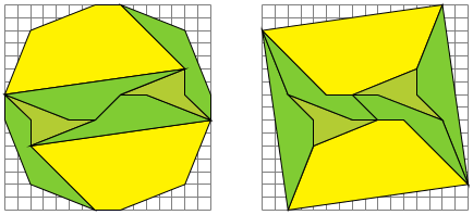
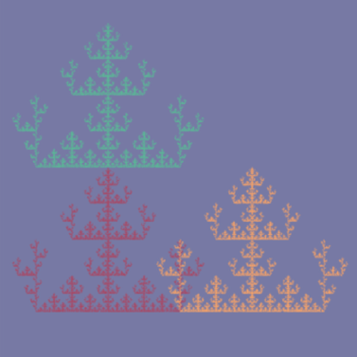
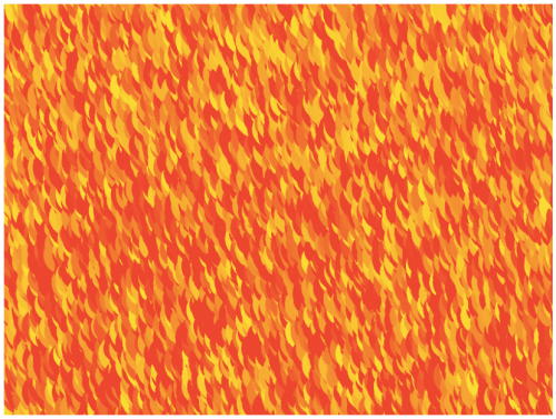
The third piece involved a color gradient (see my previous posts on Evaporation). If you look back at these posts, you’ll recall that a color gradient can be created by increasing the randomness of the colors as you move from the top of the image to the bottom using a power function: $f(y)=y$ corresponds to a linear gradient, $f(y)=y^2$ corresponds to a quadratic gradient, etc. Different effects can be created by varying the exponent.

As I was discussing this in class, one student asked what would happen if you used a negative exponent. I had never thought about this before! Jack used this idea in his piece, which he said reminds him of looking at a fire.

Day112Jack

It turns out that using a negative exponent creates a gradient beginning with black on the top. Why is this? As the image proceeds lower down the screen, the algorithm subtracts values from the RGB parameters proportional to $y^n,$ where $y=0$ corresponds to the top of the image, and $y=1$ corresponds to the bottom of the image.

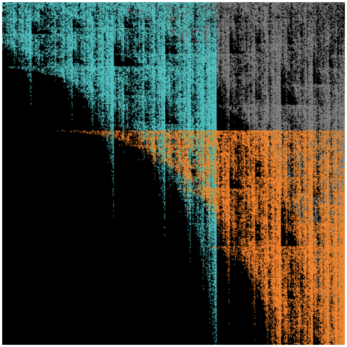
So if the exponent $n$ is positive, there is very little randomness subtracted. But if the exponent is negative, a lot of randomness is subtracted, since now the numbers near 0 are on the denominator. Because the RGB values only go up to 255, subtracting a large degree of randomness leaves nothing left — in other words, black. Now some of the numbers will end up being negative near the top– but putting all negative numbers in a color specification in Processing does in fact give you black.

Another student also worked with yellows and reds to imitate fire in another way. Instead of making small circles, he made larger circles with quite a bit of overlap, creating a rather different effect.

And Rosalie found in interesting say to create stripes with the algorithm. I had not seen this effect before.

Day112Rosalie

So that’s it for the first update of the Fall 2017 installment of Mathematics and Digital Art. As you can see, my students are already being quite creative. I look forward to seeing their work develop as the semester progresses!

Bay Area Mathematical Artists, I

Yesterday was the first meeting of the Bay Area Mathematical Artists at the University of San Francisco!

It all began one balmy Friday evening in Waterloo, Ontario, Canada at the Bridges 2017 conference….the Mendlers and I hosted a pot luck dinner at our AirBnB, and we realized how many of us were from the Bay area. In fact, we remarked upon the fact that nine of us were actually on the same flight from San Francisco to Toronto for the conference!

Bridges participants do really form a community. There is a spirit of sharing and mutual appreciation for each others’ work. We really do cherish those few days each year when we can all come together. The only drawback is that Bridges comes around just once a year.

So throughout the evening, between chowing down on grilled fare and sipping a glass of beer or wine, the idea of informally gathering now and then kept cropping up.

But as we all know, ideas do not automatically become reality. They have a tendency to wither if not watered and fertilized….so I decided to take up gardening.

I had the advantage of being associated with a University, so I could arrange a meeting space. Location was also somewhat convenient — some of us were to the northeast in Oakland and Berkeley, and others were to the southwest in Santa Clara and Scotts Valley. It might be nice to move around occasionally so not everyone has to drive as far all the time. But since the meetings are on Saturdays, at least traffic is not so much of a bother.

And then come the emails! Yes, lots of them…. The main decision to be made was deciding on a format. I thought informal was best — I sent out a call for speakers, and put them on the docket on a first-come, first-served basis. I wanted to take away the stress of competing for time; if there were more speakers than we had time for, we’d just start where we left off the last time.

The other reason for this is that I wanted to encourage students from my Mathematics and Digital Art class, as well as members of the newly formed Digital Art Club, to participate as well. I think it is important to let mathematical artists of all levels have a place to share ideas and get feedback on their work.

So for our inaugural meeting, we had three speakers: Chamberlain Fong, Karl Schaffer, and Dan Bach.

Chamberlain’s talk was entitled The Conformal Hyperbolic Square and Its Ilk. He discussed different ways to transform circular hyperbolic tilings (particularly those of Escher) to square images. Chamberlain did give a version of this talk at Bridges in 2016, but included more recent results as well. For more information, you can contact him at chamberlain@yahoo.com.

001title

Karl Schaffer’s talk was entitled Dance’s Center of Attention Mass. Inspired by Joseph Thie’s Rhythm and Dance Mathematics and Kasia Williams’ idea of “Center of Attention Mass,” Karl is interested in graphically showing where the center of attention is by weighting the position of each dancer on stage. He went so far as to contact Thie — now in his 80’s — and they are actively collaborating together.

Karl is also giving the lecture/demonstration Calculated Movements at the Montalvo Art Center next March. There is more information here. You can reach Karl at karl_schaffer@yahoo.com.

Finally, Dan Bach’s talk was entitled 3D Math Art and iBooks Author. Dan is keen on creating highly interactive math books which engage students of all ages. He gave a practical talk demonstrating the software he uses, including examples of converting graphics to various different formats since it is not always a simple task to take a 3D image created by one software package and import it into another. You can reach Dan at dan@dansmath.com.

DanBachSlide1

After the talks — which included ample room for Q&A — we had a brief discussion on the future of the group. I wanted to make it clear that while I am willing to keep things going in the current format, it is really up to the group to decide how to run our meetings. We opted to keep things going the same way for next month — but suggestions for the future included workshops, or perhaps themed sessions, like a series of talks on polyhedra. Participants were encouraged to think of other ways to use our time together as a topic of discussion for the next meeting. Keeping it informal means lessening the pressure of submitting talks/papers for conferences, etc.

Then dinner! Most of us were available for a meal afterwards. There were two nice options nearby — a cafe with sandwiches and salads, and an Indian restaurant with a buffet. I went with the group who preferred Indian food — and truly, a good time was had by all! We left for dinner at about 5:30, and I finally had to break things up shortly before 8:00, since some of us had a ways to drive home. We could clearly have kept talking for quite a while….

So our first meeting of the (tentatively named) Bay Area Mathematical Artists was a success! There were a total of 15 of us present, including three students from USF — a very respectable number for a first time event. We plan to meet approximately monthly, modulo the University schedule of classes and holidays.

I’ll post summaries each month of our meetings, including a brief synopsis of the talks, workshop(s), or whatever other form the meetings take. Feel free to contact the speakers for more information about the talks they gave this weekend, and don’t hesitate to spread the word to others who might be interested!

Using Processing for the First Time

While I have discussed how to code in Processing in several previous posts, I realized I have not written about getting Processing working on your own computer. Naturally I tell students how to do this in my Mathematics and Digital Art course. But now that I have started a Digital Art Club at the University of San Francisco, it’s worth having the instructions readily accessible.

The file I will discuss may be used to create an image based on the work of Josef Albers, as shown below.

0001

See Day002 of my blog, Josef Albers and Interaction of Color, for more about how color is used in creating this piece.

As you would expect, the first step is to download Processing. You can do that here. It may take a few moments, so be patient.

The default language used in Processing is Java. I won’t go into details of why I’m not a fan of Java — so I use Python mode. When you open Processing, you’ll see a blank document like this:

Day110Screen1

Note the “Java” in the upper right corner. Click on that button, and you should see a menu with the option “Add Mode…” Select this option, and then you should see a variety of choices — select the one for Python and click “Install.” This will definitely take a few minutes to download, so again, be patient.

Now you’re ready to go! Next, find some Processing code written in Python (from my website, or any other example you want to play around with). For convenience, here is the one I’ll be talking about today: Day03JosefAlbers.pyde. Note that it is an Open Office document; WordPress doesn’t let you upload a .pyde file. So just open this document, copy, and paste into the blank sketch. Be aware that indentation is important in Python, since it separates blocks of code. When I copied and pasted the code from the Open Office document, it worked just fine. But in case something goes awry, I always use four spaces for successive indents.

Now run the sketch (the button with the triangle pointing to the right). You will be asked to create a new folder; just say yes. When Processing runs, it often creates additional files (as we’ll see in a moment), and so keeping them all in one folder is helpful. You should also see the image I showed above; that is the default image created by this Processing program.

Incidentally, the button with the square in the middle stops running your sketch. Sometimes Processing runs into a glitch or crashes, so stopping and restarting your sketch is sometimes necessary. (I still haven’t figured out why it crashes at random times.)

Next, go to the folder that you just created. You should see a directory called “frames.” Inside, you should see some copies of the image.

Day110Screen2

Inside the “draw” function, there is a function call to “saveFrame,” which saves copies of the frames you make. You can call the folder whatever you want; this is convenient, since you might want to make two different images with the same program. Just change the folder name you save the images to.

A word about the syntax. The “####” means the frames will be numbered with four digits, as in 0001.png, 0002.png, etc. If you need more than 10,000 frames (likely you won’t when first starting), just add more hashtags. The “.png” is the type of file. You can use “.tif” as well. I use “.tif” for making movies, and “.png” for making animated gifs. There are other file types as well; see the documentation on saveFrame for more details.

Now let’s take a look at making your own image using this program.

Day110Screen3

If you notice, there are lines labelled “CHANGE 1” to “CHANGE 6” in the setup and draw functions. These are the only lines you need to change in order to design you own piece. You may tweak the other code later if you like. But especially for beginning programmers, I like to make the first examples very user-friendly.

So let me talk you through changing these lines. I won’t bother talking about the other code right now — that would take some time! But you don’t need to know what’s under the engine in order to create some interesting artwork….

CHANGE 1: The hashtags here, by the way, indicate a comment in your code: when your program runs, anything after a hashtag is ignored. This makes it easy to give hints and provide instructions in a program (like telling you what lines to change). I created a window 800 x 600 pixels; you can make it any size you want by changing those numbers. The “P2D” just means you’re working with a two-dimensional geometry. You can work in 3D in Processing, but we won’t discuss that today.

CHANGE 2: The “sqSide” variable indicates how big the square are, in units of pixels. The default unit in Processing is always pixels, so if you want to use another geometry (like a Cartesian coordinate system), you have to convert from one coordinate system to another. I do all this for you in the code; all you need to do is say how large each square is. And if you didn’t go back and read the Josef Albers piece, by “square,” I mean a unit like this:

Day002Square

CHANGE 3, CHANGE 4: The variables “sqRows” and “sqCols” indicate, as you would expect, how many rows and columns are in the final image. Since I have 15 rows and the squares are 30 pixels on a side, the height of the image is 450 pixels. Since my window is 600 pixels in height, this means there are margins of 75 pixels on the top and bottom. If your image is too tall (or too wide) for the screen, it will be cropped to fit the screen. Processing will not automatically resize — once you set the size of the screen, it’s fixed.

CHANGE 5: The “background” function call sets the color of the background, using the usual RGB values from 0-255.

CHANGE 6: The first three numbers are the RGB values of the central rectangles in a square unit. The next three numbers indicate how the background colors of the surrounding rectangles change. (I won’t go into that here, since I explain it in detail in the post on Josef Albers mentioned above. The only difference is that in that post, I use RGB values from 0-1, but in the Processing code here, I use values from 0-255. The underlying concept is the same.)

The last (and seventh) number is the random number seed. Why is this important? If you don’t say what the random number seed is (the code does involve choosing random numbers), every time you run the code you will get a different image — the computer just keeps generating more (and different) random numbers in a sequence. So if you find an image you really like and don’t know what the seed is, you’ll likely never be able to reproduce it again! And if you don’t quite like the texture created by using one random seed, you can try another. It doesn’t matter so much if you have many rows and columns, but if you try a more minimalist approach with fewer and larger squares, the random number seed makes a big difference.

OK, now you’re on your own…. This should be enough to get you started, and will hopefully inspire you to learn a lot more about Python and Processing!