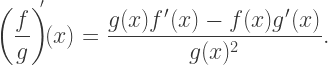
As I mentioned last week, I am a fan of emphasizing the idea of a derivative as a linear approximation. I ended that discussion by using this method to find the derivative of Today, we’ll look at some more examples, and then derive the product, quotient and chain rules.
Differentiating is particularly nice using this method. We first approximate
Then we factor out a from the denominator, giving
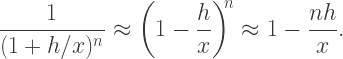
As we did at the end of last week’s post, we can make as small as we like, and so approximate by considering as the sum of an infinite series:
Finally, we have
which gives the derivative of as
We’ll look at one more example involving approximating with geometric series before moving on to the product, quotient, and chain rules. Consider differentiating We first factor the denominator:
Now approximate
so that, to first order,
This finally results in
giving us the correct derivative.
Now let’s move on to the product rule:
Here, and for the rest of this discussion, we assume that all functions have the necessary differentiability.
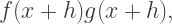
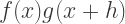
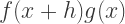
We want to approximate so we replace each factor with its linear approximation:
Now expand and keep only the first-order terms:
And there’s the product rule — just read off the coefficient of
There is a compelling reason to use this method. The traditional proof begins by evaluating
The next step? Just add and subtract (or perhaps ). I have found that there is just no way to convincingly motivate this step. Yes, those of us who have seen it crop up in various forms know to try such tricks, but the typical first-time student of calculus is mystified by that mysterious step. Using linear approximations, there is absolutely no mystery at all.
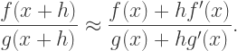
The quotient rule is next:
First approximate
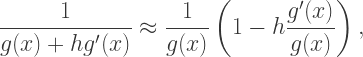
Now since is small, we approximate
so that
Multiplying out and keeping just the first-order terms results in
Voila! The quotient rule. Now usual proofs involve (1) using the product rule with and but note that this involves using the chain rule to differentiate or (2) the mysterious “adding and subtracting the same expression” in the numerator. Using linear approximations avoids both.
The chain rule is almost ridiculously easy to prove using linear approximations. Begin by approximating
Note that we’re replacing the argument to a function with its linear approximation, but since we assume that is differentiable, it is also continuous, so this poses no real problem. Yes, perhaps there is a little hand-waving here, but in my opinion, no rigor is really lost.
Since is differentiable, then exists, and so we can make as small as we like, so the “” term acts like the “” term in our linear approximation. Additionally, the “” term acts like the “” term, resulting in
Reading off the coefficient of gives the chain rule:
So I’ve said my piece. By this time, you’re either convinced that using linear approximations is a good idea, or you’re not. But I think these methods reflect more accurately the intuition behind the calculations — and reflect what mathematicians do in practice.
In addition, using linear approximations involves more than just mechanically applying formulas. If all you ever do is apply the product, quotient, and chain rules, it’s just mechanics. Using linear approximations requires a bit more understanding of what’s really going on underneath the hood, as it were.
If you find more neat examples of differentiation using this method, please comment! I know I’d be interested, and I’m sure others would as well.
In my next installment (or two or three) in this calculus series, I’ll talk about one of my favorite topics — hyperbolic trigonometry.
Last week’s post on the Geometry of Polynomials generated a lot of interest from folks who are interested in or teach calculus. So I thought I’d start a thread about other ideas related to teaching calculus.
This idea is certainly not new. But I think it is sorely underexploited in the calculus classroom. I like it because it reinforces the idea of derivative as linear approximation.
The main idea is to rewrite
as
with the note that this approximation is valid when Writing the limit in this way, we see that as a function of is linear in in the sense of the limit in the definition actually existing — meaning there is a good linear approximation to at
Moreover, in this sense, if
then it must be the case that This is not difficult to prove.
Let’s look at a simple example, like finding the derivative of It’s easy to see that
So it’s easy to read off the derivative: ignore higher-order terms in and then look at the coefficient of as a function of
Note that this is perfectly rigorous. It should be clear that ignoring higher-order terms in is fine since when taking the limit as in the definition, only one divides out, meaning those terms contribute to the limit. So the coefficient of will be the only term to survive the limit process.
Also note that this is nothing more than a rearrangement of the algebra necessary to compute the derivative using the usual definition. I just find it is more intuitive, and less cumbersome notationally. But every step taken can be justified rigorously.
Moreover, this method is the one commonly used in more advanced mathematics, where functions take vectors as input. So if
we compute
and read off
I don’t want to go into more details here, since such calculations don’t occur in beginning calculus courses. I just want to point out that this way of computing derivatives is in fact a natural one, but one which you don’t usually encounter until graduate-level courses.
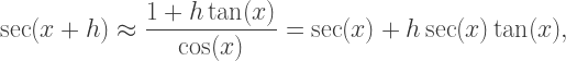
Let’s take a look at another example: the derivative of and see how it looks using this rewrite. We first write
Now replace all functions of with their linear approximations. Since and near we have
This immediately gives that is the derivative of
Now the approximation is easy to justify geometrically by looking at the graph of But how do we justify the approximation ?
Of course there is no getting around this. The limit
is the one difficult calculation in computing the derivative of So then you’ve got to provide your favorite proof of this limit, and then move on. But this approximation helps to illustrate the essential point: the differentiability of at does, in a real sense, imply the differentiability of everywhere else.
So computing derivatives in this way doesn’t save any of the hard work, but I think it makes the work a bit more transparent. And as we continually replace functions of with their linear approximations, this aspect of the derivative is regularly being emphasized.
How would we use this technique to differentiate ? We need
and so
Since the coefficient of on the left is so must be the coefficient on the right, so that
As a last example for this week, consider taking the derivative of Then we have
Now since and we have and so we can replace to get
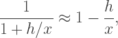
Now what do we do? Since we’re considering near then is small (as small as we like), and so we can consider
as the sum of the infinite geometric series
Replacing, with the linear approximation to this sum, we get
and so
This give the derivative of to be
Neat!
Now this method takes a bit more work than just using the quotient rule (as usually done). But using the quotient rule is a purely mechanical process; this way, we are constantly thinking, “How do I replace this expression with a good linear approximation?” Perhaps more is learned this way?
There are more interesting examples using this geometric series idea. We’ll look at a few more next time, and then use this idea to prove the product, quotient, and chain rules. Until then!
I recently needed to make a short demo lecture, and I thought I’d share it with you. I’m sure I’m not the first one to notice this, but I hadn’t seen it before and I thought it was an interesting way to look at the behavior of polynomials where they cross the x-axis.
The idea is to give a geometrical meaning to an algebraic procedure: factoring polynomials. What is the geometry of the different factors of a polynomial?
Let’s look at an example in some detail:
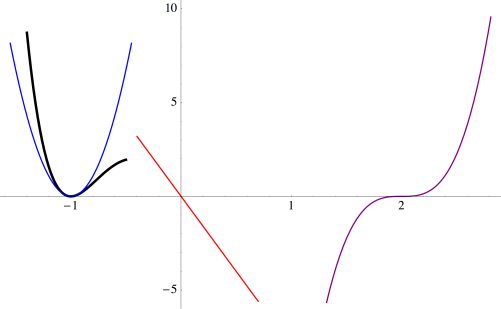
Now let’s start looking at the behavior near the roots of this polynomial.
Near the graph of the cubic looks like a parabola — and that may not be so surprising given that the factor occurs quadratically.
And near the graph passes through the x-axis like a line — and we see a linear factor of in our polynomial.
But which parabola, and which line? It’s actually pretty easy to figure out. Here is an annotated slide which illustrates the idea.
All you need to do is set aside the quadratic factor of and substitute the root, in the remaining terms of the polynomial, then simplify. In this example, we see that the cubic behaves like the parabola near the root Note the scales on the axes; if they were the same, the parabola would have appeared much narrower.
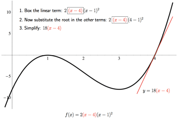
We perform a similar calculation at the root
Just isolate the linear factor substitute in the remaining terms of the polynomial, and then simplify. Thus, the line best describes the behavior of the graph of the polynomial as it passes through the x-axis. Again, note the scale on the axes.
We can actually use this idea to help us sketch graphs of polynomials when they’re in factored form. Consider the polynomial Begin by sketching the three approximations near the roots of the polynomial. This slide also shows the calculation for the cubic approximation.
Now you can begin sketching the graph, starting from the left, being careful to closely follow the parabola as you bounce off the x-axis at
Continue, following the red line as you pass through the origin, and then the cubic as you pass through Of course you’d need to plot a few points to know just where to start and end; this just shows how you would use the approximations near the roots to help you sketch a graph of a polynomial.
Why does this work? It is not difficult to see, but here we need a little calculus. Let’s look, in general, at the behavior of near the root Given what we’ve just been observing, we’d guess that the best approximation near would just be
Just what does “best approximation” mean? One way to think about approximating, calculuswise, is matching derivatives — just think of Maclaurin or Taylor series. My claim is that the first derivatives of and match at
First, observe that the first derivatives of both of these functions at must be 0. This is because will always be a factor — since at most derivatives are taken, there is no way for the term to completely “disappear.”
But what happens when the th derivative is taken? Clearly, the th derivative of at is just What about the th derivative of ?
Thinking about the product rule in general, we see that the form of the th derivative must be When a derivative of is taken, that means one factor of survives.
So when we take we also get This makes the th derivatives match as well. And since the first derivatives of and match, we see that is the best th degree approximation near the root
I might call this observation the geometry of polynomials. Well, perhaps not the entire geometry of polynomials…. But I find that any time algebra can be illustrated graphically, students’ understanding gets just a little deeper.
Those who have been reading my blog for a while will be unsurprised at my geometrical approach to algebra (or my geometrical approach to anything, for that matter). Of course a lot of algebra was invented just to describe geometry — take the Cartesian coordinate plane, for instance. So it’s time for algebra to reclaim its geometrical heritage. I shall continue to be part of this important endeavor, for however long it takes….
This week, I’ll continue with some more problems from the contests for the 2014 conference of the International Group for Mathematical Creativity and Giftedness. We’ll look at problems from the Intermediate Contest today. Recall that the first three problems on all contests were the same; you can find them here.
The first problem I’ll share is a “ball and urn” problem. These are a staple of mathematical contests everywhere.
You have 20 identical red balls and 14 identical green balls. You wish to put them into two baskets — one brown basket, and one yellow basket. In how many different ways can you do this if the number of green balls in either basket is less than the number of red balls?
Another popular puzzle idea is to write a problem or two which involve the year of the contest — in this case, 2014.
A positive integer is said to be fortunate if it is either divisible by 14, or contains the two adjacent digits “14” (in that order). How many fortunate integers n are there between 1 and 2014, inclusive?
The other two problems from the contest I’ll share with you today are from other contests shared with me by my colleagues.
In the figure below, the perimeters of three rectangles are given. You also know that the shaded rectangle is in fact a square. What is the perimeter of the rectangle in the lower left-hand corner?
I very much like this last problem. It’s one of those problems that when you first look at it, it seems totally impossible — how could you consider all multiples of 23? Nonetheless, there is a way to look at it and find the correct solution. Can you find it?
Multiples of 23 have various digit sums. For example, 46 has digit sum 10, while 8 x 23 = 184 has digit sum 13. What is the smallest possible digit sum among all multiples of 23?
You can read more to see the solutions to these puzzles. Enjoy!
As I mentioned last time, this meeting took place at Santa Clara University. As we have several participants in the South Bay area, many appreciated the shorter drive…it turns out this was the most well-attended event to date. Even better, thanks to Frank, the Mathematics and Computer Science Department at Santa Clara University provided wonderful pastries, coffee, and juice for all!
Our first speaker was Frank A. Farris, our host at Santa Clara University. (Recall that last month, he presented a brief preview of his talk.) His talk was about introducing a sound element into his wallpaper patterns.
In order to do this, he used frequencies based on the spectrum of hexagonal and square grids. It’s not important to know what this means — the main idea is that you get frequencies that are not found in western music.
Frank’s idea was to take his wallpaper patterns, and add music to them using these non-traditional frequencies. Here is a screenshot from one of his musical movies:
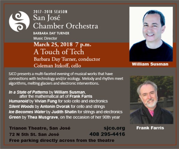
Frank was really excited to let us know that the San Jose Chamber Orchestra commissioned work by composer William Susman to accompany his moving wallpaper patterns. The concert will take place in a few weeks; here is the announcement, so you are welcome to go listen for yourself!
Frank has extensive information about his work on his website http://math.scu.edu/~ffarris/, and even software you can download to make your very own wallpaper patterns. Feel free to email him with any questions you might have at ffarris@scu.edu.
The second talk, Salvador Dali — Old and New, was given by Tom Banchoff, retired from Brown University. He fascinated us with the story of his long acquaintance with Salvador Dali. It all began with an interview in 1975 with the Washington Post about Tom’s work in visualizing the fourth dimension.
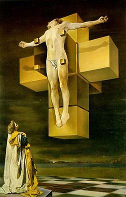
He was surprised to see that the day after the interview, the article Visual Images And Shadows From The Fourth Dimension in the next day’s Post, as well as a picture of Dali’s Corpus Hypercubus (1954).
Salvador Dali’s Crucifixion (Corpus Hypercubus)
But Tom was aware that Dali was very particular about giving permission to use his work in print, and knew that the Post didn’t have time to get this permission in such a short time frame.
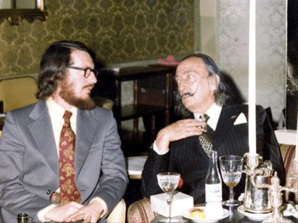
The inevitable call came from New York — Dali wanted to meet Tom. He wondered whether Dali was simply perturbed that a photo of his work was used without permission — but luckily, that was not the reason for setting up the meeting at all. Dali was interested in creating stereoscopic oil paintings, and stereoscopic images were mentioned in the Post article.
Thus began Tom’s long affiliation with Dali. He mentioned meeting Dali eight or nine times in New York (Dali came to New York every Spring to work), three times in Spain, and once in France. Tom remarked that Dali was the most fascinating person he’d ever met — and that includes mathematicians!
Tom with Salvador Dali.
Then Tom proceeded to discuss the genesis of Corpus Hypercubus. His own work included collaboration with Charles Strauss at Brown University, which included rendering graphics to help visualize the fourth dimension — but this was back in the 1960’s, when computer technology was at its infancy. It was a lot more challenging then than it would be today to create the same videos.
Tom’s rendition of a hypercube net.
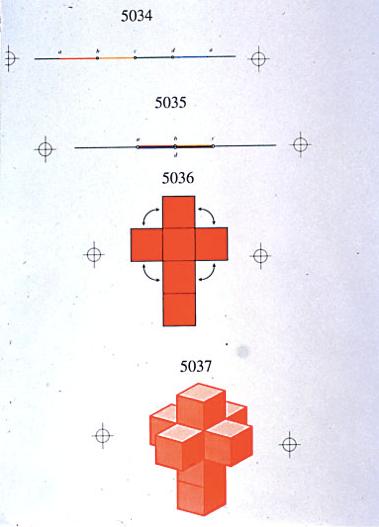
He also spent some time discussing a net for the hypercube, since a hypercube net is the geometrical basis for Dali’s Corpus Hypercubus. What makes understanding the fourth dimension difficult is imagining how this net goes together.
It is not hard to imagine folding a flat net of six squares to make a cube — but in order to do that, we need to fold some of the squares up through the third dimension. But to fold the hypercube net to make a hypercube without distorting the cubes requires folding the cubes up into a fourth spatial dimension.
This is difficult to imagine! Needless to say, this was a very interesting discussion, and challenged participants to definitely think outside the box.
Tom remarked that Dali’s interest in the hypercube was inspired by the work of Juan de Herrera (1530-1597), who was in turn inspired by Ramon Lull (1236-1315).
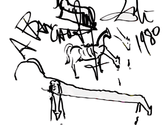
Tom also mentioned an unusual project Dali was interested in near the end of his career. He wanted to design a horse that when looked at straight on, looks like a front view of a horse. But when looked from the side, it’s 300 meters long! For more information, feel free to email Tom at banchoff@math.brown.edu.
Dali’s sketch of the horse.
Suffice it to say that we all enjoyed Frank’s and Tom’s presentations. The change of venue was welcome, and we hope to be at Santa Clara again in the future.
Following the talks, Frank generously invited us to his home for a potluck dinner! He provided lasagna and eggplant parmigiana, while the rest of us provided appetizers, salads, side dishes, and desserts.
As usual, the conversation was quite lively! We talked for well over two hours, but many of us had a bit of a drive, so we eventually needed to make our collective ways home.
Next time, on April 7, we’ll be back at the University of San Francisco. At this meeting, we’ll go back to shorter talks in order to give several participants a chance to participate. Stay tuned for a summary of next month’s talks!
The Regional Meeting of the Golden Section of the Mathematical Association of America was held at California State University, East Bay. The local organizer was Shirley Yap, fellow mathematical artist, who deserves kudos for the monumental amount of work it takes to organize a conference like this! I helped out by organizing this year’s Art Exhibition.
This year, I thought I’d give you a virtual tour of the exhibit! So I asked contributing artists to submit their own personal statement about their work and/or mathematical art in general, as well as an image of one of their displayed artworks. I’ll let the artists speak for themselves…. (By the way, the order the artists are presented in is the order in which they sent me their information. There is no ranking implicit in the order.)
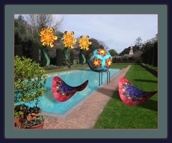
I created this image out of golden spirals. While working on a math demonstration for my students, I unpacked a roll of netting. During the unraveling process, I had a vision of a two-dimensional golden spiral unravelling, which I tried to recreate with code. I wanted to viewer to not just witness the unraveling, but also be inside the web of the fabric. I often create code that has a lot of randomness in it, so that it captures a moment in time that can never be recreated.
Mathematicians can feel lonely to find ourselves face to face with the most beautiful thoughts humans have ever known, only to realize that communicating our experience is unreasonably difficult. I have found comfort in visual art, digitally computed images that are the best I can do (short of giving an hour lecture) to say, ‘This is the beauty of mathematics.’
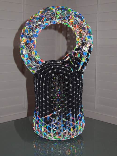
I’m primarily a middle school mathematics teacher with one of my hobbies being Origami and other paper crafts. Some years back I became interested in the work of Heinz Strobl which uses joined, folded strips of paper to create various structures. Much like unit origami, the structures are held together solely by the folds, no adhesives. My interest soon became an obsession and I’ve been neck-deep in little strips of paper ever since. Lately I’ve been exploring concepts in Topology. This particular work is my attempt at a Klein Bottle.
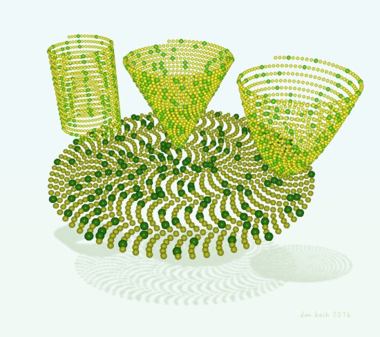
“I’m a career college mathematics teacher, now an interactive book author and 3D math artist. I like to illustrate number theory and vector calculus principles with surprising and colorful images, using a software palette of Mathematica, Cheetah3D, and iBooks Author. My math art encourages viewers to think, notice, and wonder. And hopefully say, ‘That’s cool! That’s math?’ “
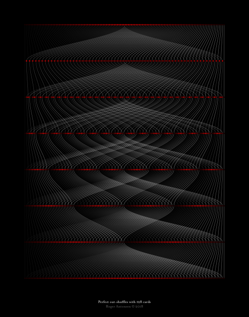
This is a visualization of seven repeated perfect out-shuffles of a deck with 128 cards. The horizontal lines represent the particular orders of the cards throughout the shuffling, and the vertical curves represent the path each card takes from start to finish. The curves are colored from black to white in order to show the mechanics of the shuffling. The dots are colored from black to red to black in order to show that each perfect out-shuffle preserves the so-called “stay-stack principle”. Notice that the order of cards returns to the original order after seven shuffles.
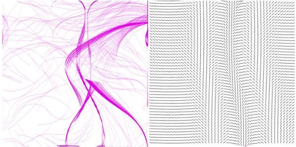
This image is an embedding of a photograph of a set of watercolors. The embedding was performed using Locally Linear Embedding (LLE), a nonlinear dimensionality reduction technique, introduced by Saul & Roweis in 2000. LLE is an unsupervised machine learning algorithm.
I am pursuing a double major in Mathematics and Computer Science. I am currently working on research in geometric dimensionality reduction and unsupervised machine learning. This work will be extended into neural networks and deep learning. I enjoy seeking out interesting intersections between mathematics, computer science, and art.
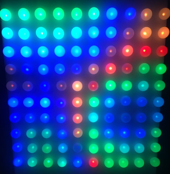
Undulating organic light show with minimal code generated by a 16 MHz processor calculating color and brightness values through a Perlin noise algorithm. Blobs appear to grow, shrink, and drift relaxingly over the LED grid. 100 ping pong balls covering 100 individually addressable LEDs on poster board with Arduino Nano v.3 controller and battery pack.
Programming is my art. I might not be a good “designer”, but I am a good developer where I am able to take a structured approach on art. I specialize in computer graphics, thus my understanding of the mathematics behind geometry, 3D models, and 2D sprites are better than my ability to free-form draw them.
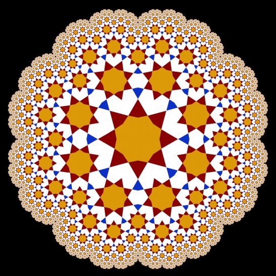
All of my work stems from one core impulse: to celebrate the inherent beauty of mathematical forms. Since traveling to India in 2012, I have been particularly focused on blending traditional Islamic motifs with polyhedra and fractals. The results are distinctly Islamic in flavor but with a modern twist.
This piece has global and local 8-fold rotational symmetry around each gold star. Star centers occupy the nodes of 8 fractal quaternary trees, which are pruned at the octant boundaries. The original central star is replaced by an inward progression of the same fractal diminution.
This piece is based on fractal binary trees. The usual way of creating a binary tree is to move forward, then branch to the left and right some fixed angle as well as shrink, and repeat recursively. Recent work involves specifying the branching by arbitrary affine transformations. In this piece, the affine transformations were chosen so that as the tree grows, nodes are repeatedly visited. The nodes are covered by disks which become smaller with each iteration, accounting for the overlapping circles. The research needed to produce these images was undertaken jointly with Nick Mendler.
I hope you enjoyed this virtual tour of the Art Exhibition at the recent MAA Regional Conference. The upcoming conference is next March; stay tuned for another virtual tour in about a year!
In going through some folders in my office the other day, I came across some sets of mathematics puzzles I wrote for a conference of the International Group for Mathematical Creativity and Giftedness in 2014. Teachers of mathematics of all levels attended, from elementary school to university. The organizing committee (which included me) thought it might be fun to have some mathematical activity that conference attendees could participate in.
So I and my colleagues created three levels of contests — Beginning, Intermediate, and Advanced — since it seemed that it would be difficult to create a single contest that everyone could enjoy. But I did include three problems that were the same at every level, so all participants could talk about some aspect of the contests with each other.
Participants had a few days to get as many answers as they could, and we even had books for prizes! Many remarked how much they enjoyed working out these puzzles.
Now this conference took place before I started writing my blog. I have written several similar contests over the years for various audiences, and so I thought it would be nice to share some of my favorite puzzles from the contests with you. And so The Puzzle Archives are born!
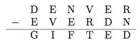
First, I’ll share the three puzzles common to all three contests. I needed to create some puzzles which were fun, and didn’t require any specialized mathematical knowledge. As I’m a fan of cryptarithms and the conference took place in Denver, I created the following puzzle. Here, no letter stands for the digit “0.”
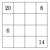
For the next puzzle, all you need to do is complete the magic square using the even numbers from 2 to 32. Each row, column, and diagonal should add up to the same number. There are two solutions to this puzzle — and so you need to find them both!
And of course, I had to include one of my favorite types of puzzles, a CrossNumber puzzle. Remember, no entry in a CrossNumber puzzle can begin with “0.”
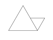
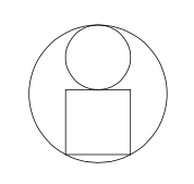
I also included a few geometry problems, staples of any math contest. For the first one, you need to find the area of the smallest circle you could fit the following figure into. Both triangles are equilateral; the smaller has side length 1 and the larger has side length 2.
And for the second one, you need to find the radius of the larger circle. You are given that the smaller circle has a diameter of 2 units, and the sides of the square are 2 units long. Moreover, the smaller circle is tangent to the square at the midpoint of its top edge, and is also tangent to the larger circle.
The last two problems I’ll share from this contest are number puzzles. The first is a word problem, which I’ll include verbatim from the contest itself.
Tom and Jerry each have a bag of marbles. Tom says, “Hey, Jerry. I have four different colors of marbles in my bag. And the number of each is a different perfect square!” Jerry says, “Wow, Tom! I have four different colors of marbles, too, but the number of each of mine is a different perfect cube!”
If Tom and Jerry have the same total number of marbles, what is the least number of marbles they can have?
And finally, another cryptarithm, but with a twist. In the following multiplication problem, F,I,N, and D represent different digits, and the x‘s can represent any digit. Your job is to find the number F I N D. (And yes, you have enough information to solve the puzzle!)
Happy solving! You can read more to see the solutions; I didn’t want to just put them at the bottom in case you accidentally saw any answers. I hope you enjoy this new thread!
(Note: The FIND puzzle was from a collection of problems shared by a colleague. The first geometry problem may have come from elsewhere, but after four years, I can’t quite remember….) Continue reading The Puzzle Archives, I
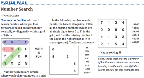
Last fall, I mentioned that while looking at the Puzzle Page of the FOCUS magazine published by the Mathematical Association of America, I thought to myself, “Hey, I write lots of puzzles. Maybe some of mine can get published!” So I submitted a few Number Search puzzles to the editor, and to my delight, she included them in the December/January issue. Here’s the proof….
Incidentally, these puzzles are the same ones I wrote about almost two years ago — hard to believe I’ve been blogging that long! So if you want to try them, you can look at Number Searches I and Number Searches II.
Since I had success with one round of puzzles, I thought I’d try again. This time, I wanted to try a few CrossNumber puzzles (which I wrote about on my third blog post). But as my audience was professional mathematicians and mathematics teachers, I wanted to try to come up with something a little more interesting than the puzzles in that post.
To my delight again, my new trio of puzzles was also accepted for publication! So I thought I’d share them with you. (And for those wondering, the editor does know I’m also blogging about these puzzles; very few of my followers are members of the MAA….)
Here is the first puzzle.
Answers are entered in the usual way, with the first digit of the number in the corresponding square, then going across or down as indicated. In the completed puzzle, every square must be filled.
I thought this was an interesting twist, since every answer is a different power of an integer. I included this as the “warmup” puzzle. It is not terribly difficult if you have some software (like Mathematica) where you can just print out all the different powers and see which ones fit. There are very few options, for example, for 3 Down.
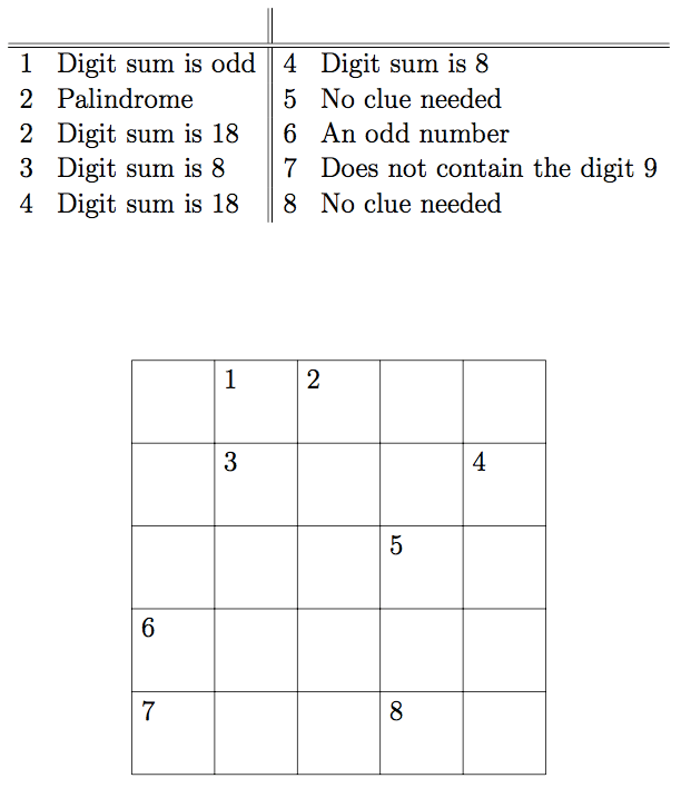
The next puzzle is rather more challenging!
All the answers in this puzzle are perfect cubes with either three or four digits, and there are no empty squares in the completed puzzle. But you might be wondering — where are the Across and Down clues? Well, there aren’t any….
In this puzzle, the number of the clue tells you where the first digit of the number goes — or maybe the last digit. And there’s more — the number can be written either horizontally or vertically — that’s for you to decide! So, for example, if the answer to Clue 5 were “216,” there would be six different ways you could put it in the grid: the “2” can go in the square labelled 5, and the number can be written up, down, or to the left. Or the “6” can go in the square labelled 5, again with the same three options.
This makes for a more challenging puzzle. If you want to try it, here is some help. Let me give you a list of all the three- and four-digit cubes, along with their digit sum in parentheses: 125(8), 216(9), 343(10), 512(8), 729(18), 1000(1), 1331(8), 1728(18), 2197(19), 2744(17), 3375(18), 4096(19), 4913(17), 5832(18), 6859(28), 8000(8), 9261(18). And in case you’re wondering, a number which is a palindrome reads the same forwards and backwards, like 343 or 1331.
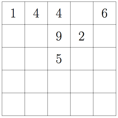
The third puzzle is a bit open-ended.
To solve it, you have to fill each square with a digit so that you can circle (word search style) as many two- and three-digit perfect squares as possible. In the example above, you would count both 144 and 441, but you would only count 49 once. You could also count the 25 as well as the 625.
I don’t actually know the solution to this puzzle. The best I could do was fill in the grid so I could circle 24 out of the 28 eligible perfect squares between 16 and 961. In my submission to MAA FOCUS, I ask if any solver can do better. Can you fit more than 24 perfect squares in the five-by-five grid? I’d like to know!
I’m very excited about my puzzles appearing in a magazine for mathematicians. I’m hoping to become a regular contributor to the Puzzle Page. It is fortunate that the editor likes the style of my puzzles — when the magazine gets a new editor, things may change. But until then, I’ll need to sharpen my wits to keep coming up with new puzzles!
The Spring semester is now well underway! This means it’s time for the Bay Area Mathematical Artists to begin meeting. This weekend, we had our first meeting of 2018 at the University of San Francisco.
As usual, we began informally at 3:00, giving everyone plenty of time to make it through traffic and park. This time we had three speakers on the docket: Frank A. Farris, Phil Webster, and Roger Antonsen.
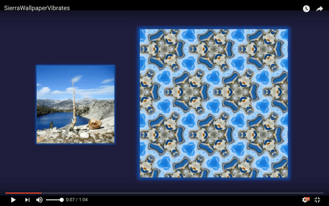
Frank started off the afternoon with a brief presentation, giving us a teaser for his upcoming March talk on Vibrating Wallpaper. Essentially, using the complex analysis of wave forms, he takes digital images and creates geometrical animations with musical accompaniment from them. A screenshot of a representative movie is shown below:
You can click here to watch the entire movie. More details will be forthcoming in the next installment of the Bay Area Mathematical Artists (though you can email him at ffarris@scu.edu if you have burning questions right now). Incidentally, the next meeting will be held at Frank’s institution, Santa Clara University; he has generously offered to host one Saturday this semester as we have several participants who drive up from the San Jose area.
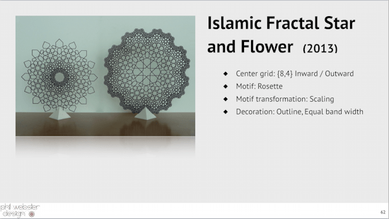
Our second speaker was Phil Webster, whose talk was entitled A Methodology for Creating Fractal Islamic Patterns. Phil has been working with Islamic patterns for about five years now, and has come up with some remarkable images.
Here, you can see rings of 10 stars at various levels of magnification, all nested very carefully within each other. While it is fairly straightforward to iterate this process to create a fractal image, a difficulty arises when the number and size of rosettes at a given level of iteration are such that they start overlapping. At this point, a decision must be made about which rosettes to keep.
This decision involves both mathematical and artistic considerations, and is not always simple. One remark Phil hears fairly often is that he’s actually creating a model of the hyperbolic plane, but this is in fact not the case. Having sat down with him while he explained his methodology to me, I can attest to this fact. His work may be visually somewhat reminiscent of the hyperbolic plane, but the mathematics certainly is not.
Moreover, in addition to creating digital prints, Phil has also experimented with laser cutting Islamic patterns, as shown in the intricate pieces below.
If you would like to learn more about Phil’s Islamic fractal patterns, feel free to email him at phil@philwebsterdesign.com.
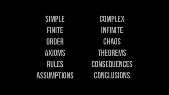
We ended with a talk by Roger Antonsen, From Simplicity to Complexity. Roger is giving a talk at the Museum of Mathematics in New York City next month, and wanted a chance to try out some ideas. He casually remarked he had 377 slides prepared, and indicated he needed to perhaps trim that number for his upcoming talk….
Roger remarked that as mathematicians, we know on a hands-on basis how very simple ideas can generate enormous complexity. But how do you communicate this idea to a general audience, many who are children? This is his challenge.
The idea of this “tryout” was that Roger would share some of his ideas with us, and we would give him some feedback on what we thought. One idea that was very popular with participants was a discussion of Langton’s ant. There are several websites you can visit — but to see a quick overview, visit the Wikipedia page.
The rules are simple (as you will already know if you googled it!). An ant starts on a grid consisting totally of white squares. If the ant is on a white square, it turns right a quarter-turn, moves ahead one square, and the square the ant was on turns to black. But if the ant is on a black square, it turns left a quarter-turn, moves one unit, and the square the ant was on turns to white.
It seems like a fairly simple set of rules. As the ant starts moving around, it seems to chaotically color the squares black and white in a random sort of pattern.
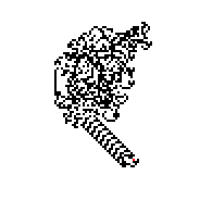
From the Wikipedia commons, user Krwawobrody.
The image above shows the path of the ant after 11,000 steps (with the red pixel being the last step). Notice that the path has started to repeat, and continues to repeat forever!
Why? No one really knows. Yes, we can see that it actually does repeat, but only sometime after 10,000 apparently random steps. The behavior of this system has all of a sudden become very mysterious, without a clear indication of why.
If the rules for moving the ant always resulted in just random-looking behavior, perhaps no one would have looked any further. But there are so many surprises. Especially since there is no reason you have to stick to the rules above. As suggested in the Wikipedia article, you can add more colors, more rules, and even more ants….
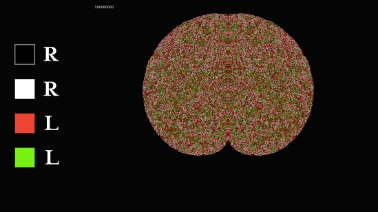
For example, consider the set of rules in the following image. It should be relatively self-explanatory by now: there are four colors; if the ant is on a black square, turn right a quarter-turn and move forward one unit, then change the color of the square the ant was on to white; then continue (where green squares becomes black, in cyclic order).
This looks like a cardiod! And if you actually zoom in enough, you’ll see that this is the image after 500,000,000 iterations…though again, no one has the slightest idea why this happens. Why should a simple set of rules based on 90° rotations generate a cardioid, of all things?
From the simple to the complex! This was only one of literally dozens of topics Roger was able to elaborate on — and he illustrated each one he showed us with compelling images and animations. For more examples, please see his web page, or feel free to email him at rantonse@ifi.uio.no. You can also see the announcement for his MoMath talk here.
As usual, we went our for dinner afterwards, this time for Thai. It seems that no one wanted to leave — but some of the participants had a 90-minute drive ahead of them, so eventually we had to head home. Stay tuned for the summary of next month’s meeting, which will be at Santa Clara University!
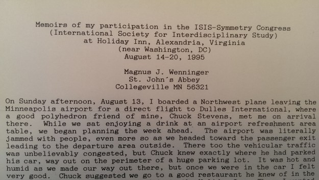
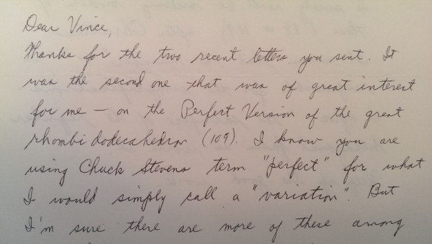
This is the final installment about my correspondence with Magnus Wenninger. I didn’t realize I had so much to say! But I am glad to take the opportunity to share a bit about a friend and colleague who contributed so much to the revitalization of three-dimensional geometry in recent years. Talk to anyone truly interested in polyhedra, and they will know of Magnus.
Excerpt from 14 August 1995.
As I mentioned last week, I’ll begin with Magnus’ memoir on the Symmetry Congress (as you can see in the title of his memoir). His friend Chuck Stevens lived near where the Congress was held, and so met him at the airport and was his tour guide for the duration of his visit. (Note: the Society is still active — just google it!)
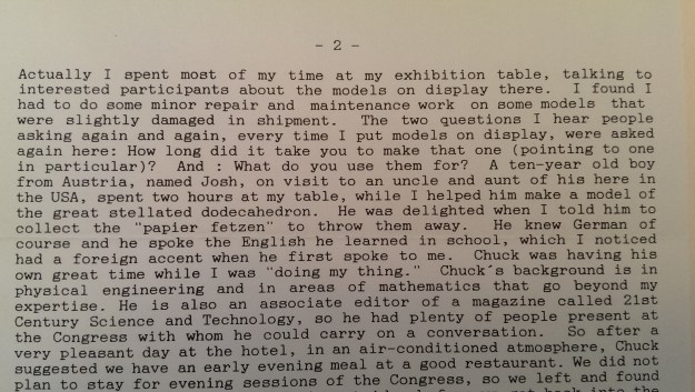
Excerpt from 14 August 1995.
In this excerpt, Magnus remarks (start in the middle of line 4) that people who don’t know much about polyhedra always ask the same two questions: how long did it take you to make that model, and what do you do with them? I have had similar questions asked of me over the years as well; you just learn to be patient and hopefully enlighten…. Of course Magnus was always kind and generous with his responses.
You might be surprised by Magnus talking with a 10-year-old boy at the conference. Of course it may have been that Josh just happened to be staying at the same hotel, though that is unlikely since he was visiting relatives. More likely is that his aunt or uncle was a conference participant and brought him to the conference. I should remark that it is a common occurrence for a participant in an international conference to plan a family vacation around the trip, so you regularly see children of all ages at such conferences.
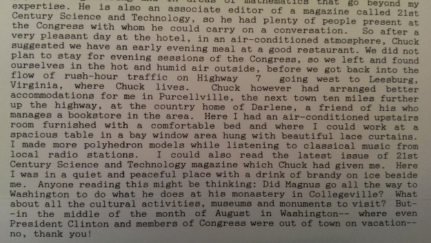
Excerpt from 14 August 1995.
I direct your attention to last seven lines here. Magnus was perfectly happy to have his brandy, building polyhedra in an air-conditioned room rather than braving the summer heat to be “cultural.” For me, this emphasizes the simplicity of Magnus’ life. He did not need much to make him happy — some paper and glue, his building tools, his Bible, and perhaps a few other books on philosophy and theology. The quintessential minimalist life of a Benedictine monk.
Excerpt from 14 August 1995.
Here, the second paragraph is interesting. In rereading it, I think I could imagine the exact expression on Magnus’ face when he heard “I’ll take it.” I know that this was a rare occurrence for Magnus. Perhaps it might be less so now; because of Magnus’ influence, as well as the explosion of computer graphics on the internet, people are generally more informed about polyhedra than they were in 1995.
Moreover, more and more high school geometry textbooks are moving away from exclusively two-column proofs, and some even have chapters devoted to the Platonic solids. I don’t think we’re at the point yet where “dodecahedron” is a household word…but we’re definitely moving, if slowly, closer to that point.
Excerpt from 4 December 1995.
The final excerpt I’d like to share is from December 1995. I include this as another example of my collaboration with Magnus — our discussions of “perfect versions” of polyhedra. I’ll go into this example in more detail since it’s a bit easier to understand, but I note Magnus was not a fan of the adjective “perfect.” (And as a historical note, I had used the term “perfect version” and had also corresponded with Chuck Stevens, so Chuck must subsequently have talked to or corresponded with Magnus and used the term, and so Magnus thought Chuck came up with the term.)
I now agree, but have yet to come up with a better term. The basic idea is that some polyhedron models are very complicated to build. But for many of them, there are ways to make similar-looking polyhedra which are still aesthetically pleasing, but a bit easier to construct.
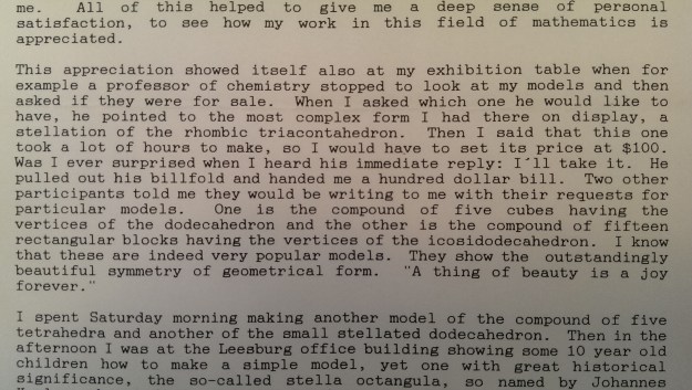
Let’s look at an example I mentioned a few weeks ago: the stellated truncated hexahedron, shown below.
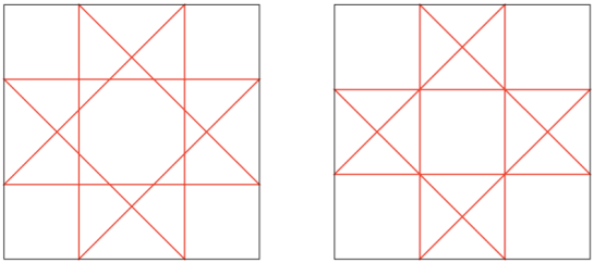
Notice the blue regular octagrams. Now consider the octagrams shown here.
On the left is a regular octagram. If you draw a square around it, as shown, you divide the edges of the square in the ratio Notice that the octagram is divided into 17 smaller pieces by its edges.
However, if you start with a square and subdivide the edges into equal thirds, an interesting phenomenon occurs — there are four points where three edges intersect, resulting in a subdivision of the octagram into just 13 pieces.
You will note that this variation is not regular — the horizontal and vertical edges are not the same length as the diagonal edges. So any polyhedron with this octagram as a face would not be a uniform polyhedron.
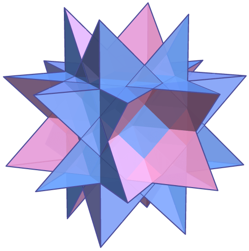
However, it would be what Magnus referred to as a “variation” of a uniform polyhedron. So if we took the stellated truncated hexahedron, kept the planes containing the pink triangles just where they are, but slightly move the planes containing the blue octagrams toward the center, we would end up with the following polyhedron:
Note that the octagrams are now the octagram variations. Also notice how the pentagonal visible pink pieces are now rhombi, and the small blue square pieces are completely absent!
Such simplifications are typical when working with this kind of variation. Of course many polyhedra have such variations — but now isn’t time to go into further details. But these variations were among the polyhedra Magnus and I wrote about.
As I mentioned, there is little left of my correspondence with Magnus, since several years of emails have been lost. But I hope there is enough here to give you a sense of what Magnus was like as an individual, friend, and colleague. He never let his fame or reputation go to his head — all he was ever doing, as he saw it, was taking an idea already in the mind of God, and making it real.
He truly was humble, gentle, and kind — and of course a masterful geometer who significantly influenced the last few generations of polyhedron model builders. He will be missed.


 Writing the limit in this way, we see that
  as a function of
  is linear in

 This is not difficult to prove.
 It’s easy to see that
 to the limit. So the coefficient of
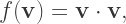


 and see how it looks using this rewrite. We first write
 and
and  near
near  we have

 But how do we justify the approximation
 at
at  does, in a real sense, imply the differentiability of
  ? We need

 so must be the coefficient on the right, so that
 Then we have
 we have
  and so we can replace to get
 then
then  is small (as small as we like), and so we can consider


 to be
to be

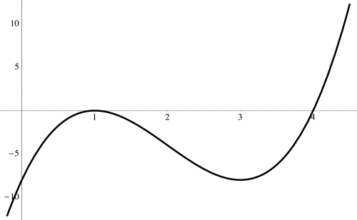
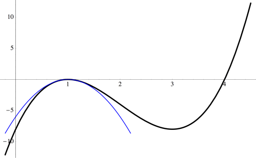
 the graph of the cubic looks like a parabola — and that may not be so surprising given that the factor
  occurs quadratically.
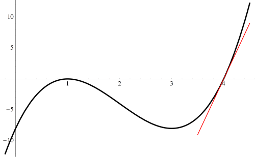
 the graph passes through the x-axis like a line — and we see a linear factor of
  in our polynomial.
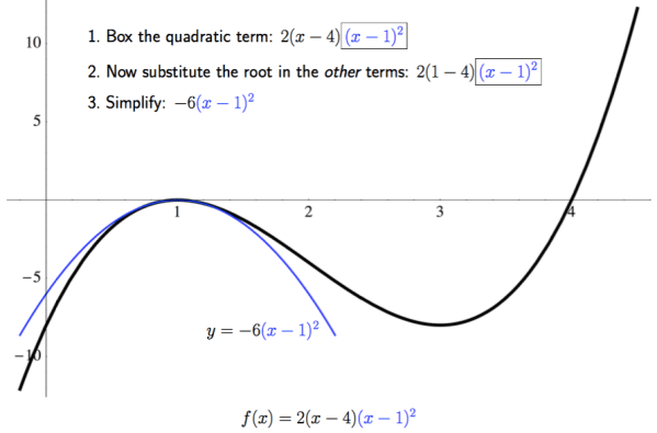
 and substitute the root,
  near the root
  Note the scales on the axes; if they were the same, the parabola would have appeared much narrower.
 substitute
  in the remaining terms of the polynomial, and then simplify. Thus, the line
  best describes the behavior of the graph of the polynomial as it passes through the x-axis. Again, note the scale on the axes.
 Begin by sketching the three approximations near the roots of the polynomial. This slide also shows the calculation for the cubic approximation.
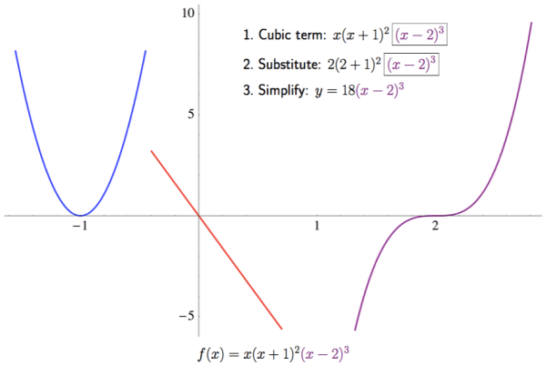

 Of course you’d need to plot a few points to know just where to start and end; this just shows how you would use the approximations near the roots to help you sketch a graph of a polynomial.
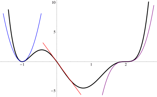
 near the root
  Given what we’ve just been observing, we’d guess that the best approximation near
  would just be
 derivatives of
  match at
  derivatives of both of these functions at
  will always be a factor — since at most
  term to completely “disappear.”
 at
at  What about the
  When a derivative of
  is taken, that means one factor of
  we also get
 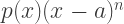 and
and 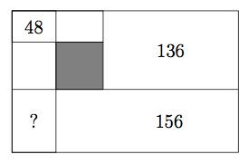


 Notice that the octagram is divided into 17 smaller pieces by its edges.