Now that I’ve talked about what I use computer graphics for in my last installment of On Coding, I’d like to talk about the most useful graphics package I’ve come across for writing mathematics: TikZ.
First a word about the name, TikZ. It’s an example of a recursive acronym, like GOD used in Douglas Hofstadter’s Gödel, Escher, Bach, which stands for “GOD Over Djinn.” (By the way, read Gödel, Escher, Bach if you haven’t already — it’s an amazing book about Gödel’s Incompleteness Theorem.)
So TikZ stands for “TikZ ist kein Zeichenprogramm,” which is German for “TikZ is not a drawing program.” According to its creator, Till Tantau, this indicates that TikZ is not a way to draw pictures with your mouse or tablet, but is more like a computer graphics language. It is designed for use in LaTeX, and is built with a lower-level language called PGF, which stands for “portable graphics format.”
So enough history — you can read more in the TikZ manual. But a word of caution — it’s over 1000 pages long, so there’s a lot there! I’ll only be able to scratch the surface today.
The two most important features of TikZ, in my opinion, are (1) you can draw very precise graphics because you’re writing in a high-level langauge, not using a WYSIWYG environment, and (2) you can use it in LaTeX, including putting any LaTeX symbols in your graphics. This second point is extremely important, since it means when you’re labelling a diagram, the labels (usually involving mathematical symbols) look exactly the same way as the do in your text.
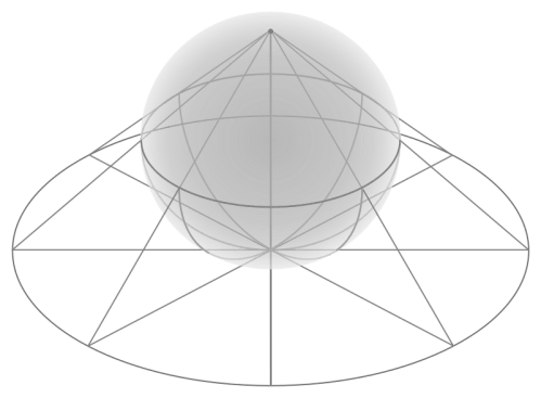
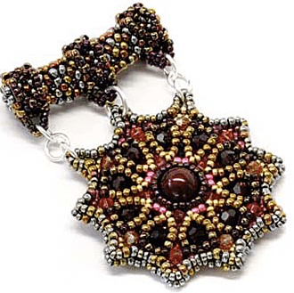
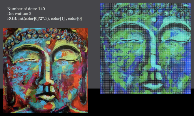
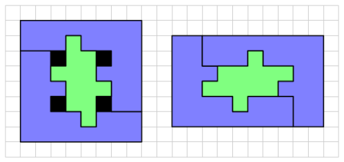
I use TikZ almost exclusively for two-dimensional mathematical graphics. In a recent paper, for example, I created the following image.
Note how precisely all the elements are rendered — this is because you give precise coordinates for all the individual graphics elements.
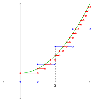
Let’s take a look at another, somewhat simpler example from this paper.
I chose this example for a few reasons. First, it requires using a lot of the basic TikZ commands. Second, it illustrates the practical side of drawing computer graphics. No, I’m not going to submit this image to a Bridges art exhibition any time soon — but if I need to make an image for a paper, I want it to look good.
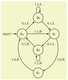
So I thought I’d take some time to explain various aspects of the code which creates this image. Maybe not the most glamorous graphic — but you’re welcome to look at the 1000+ page manual for hundreds of neat examples. Here is a diagram for a finite-state automaton from page 179, for example.
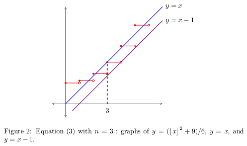
Here’s what you’d need to type in LaTeX to get the simple graph I mentioned a moment ago.
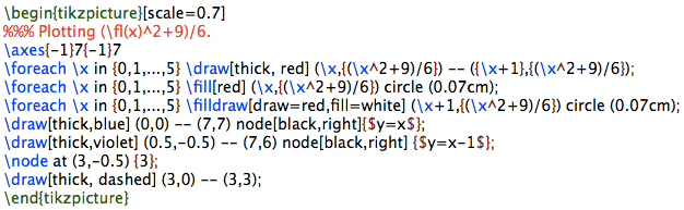
Let’s look at several different excerpts from this example. The first line opens your TikZ environment, and scales the image. The default unit is 1 cm, so you need to set the scale to get your image the right size.
The next line is just a comment — I don’t use comments much for simple images. But for more complex images, they’re important. Just as important as commenting computer code.
The next line draws a set of axes. What’s important here is that I defined my own “\axes” command — so you can include user-defined functions as well. The advantages of being able to do this are huge. You can use any command you define in LaTeX in a TikZ image.
Another great feature is the looping construct, “\foreach.” The red segments above are one unit long, and so the only difference is the starting points. Also important here is that you can use mathematical expressions inside TikZ, like the “{(\x^2+9)/6}” expression in the curly brackets.
Note the directives “[thick, red]” after the “draw” command. You have control over every aspect of the drawing routines in TikZ — and there are lots of them. For example, there is the “dashed” directive in line 10. But not only can you draw a dashed line, but you can also specify the lengths of the dash marks and the spaces between them, too! Further, you can create user-defined styles if you use the same set of directives over and over again. This is helpful if you are creating several related images, and you want to tweak the color, for example. You only have to change the color specification in the style, and every image which uses that style will be rendered using the new color.
Notice the “\filldraw” command in line 6. I wanted open circles, so I drew the circles in red, and filled them with white. If I wanted to, I could have also specified precisely how thick I wanted the circles to be drawn, but the default thickness looked just fine to me.
Notice the use of “node” and “\node” throughout. In line 9, for example, the “3” is centered at coordinates (3, -0.5). Also note the placement of nodes at the end of line segments, as shown in lines 7 and 8. Again, it is significant that you can include any text you can create in LaTeX in your diagram.
I hope this is enough to give you the feel of using TikZ. As I mentioned in the last installment, I also use TikZ to create slideshow presentations since there is so much you can do. Remember, there are over 1000 pages of examples of things you can do in TikZ in the manual.
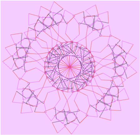
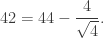
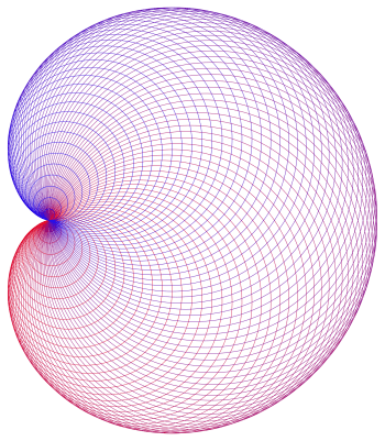
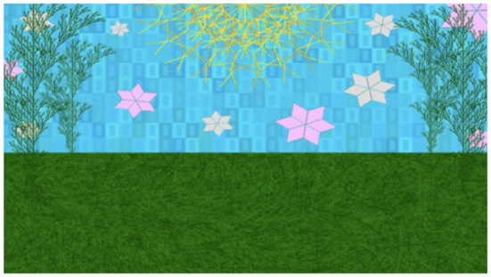
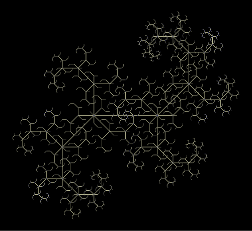
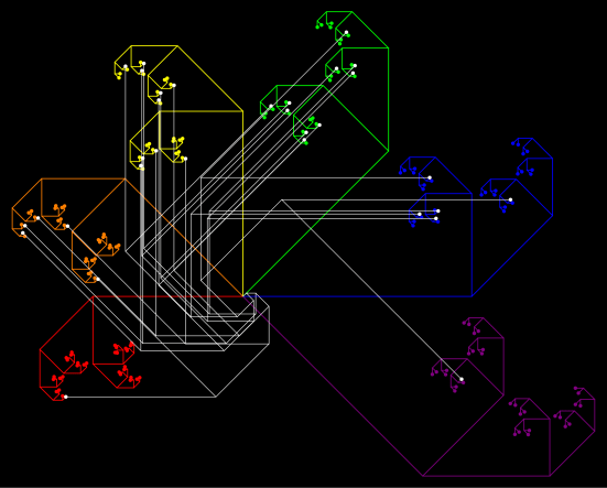
I would like to mention one caveat, however. I do sometimes use Mathematica to create images with mathematically intensive equations and calculations. TikZ is closer to a markup language in its usage, as I see it — so any image that requires significant coding to produce is a bit too cumbersome syntactically. Here is an example of an image I used Mathematica to create.

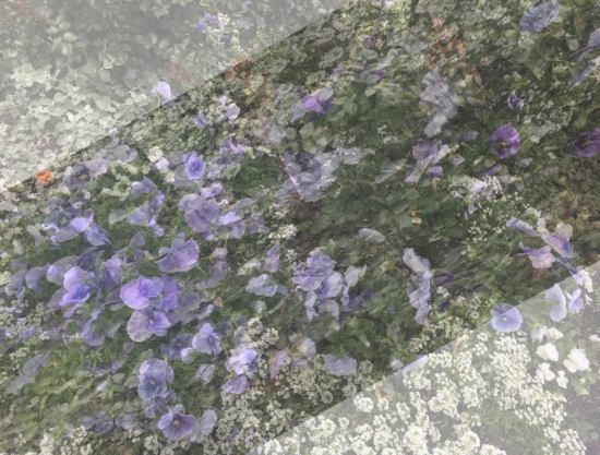
But another nice TikZ feature is that you can import images into your environment — so I can draw complex images in Mathematica, include them in my TikZ picture, and then overlay LaTeX symbols on top of the image. With this capability, the possibilities are quite literally endless.
A final comment: TikZ and LaTeX are both open source, so if you’re interested, you can just download them and start experimenting! The learning curve is a little steep, admittedly, but once you’ve climbed up, you’ll be able to create astonishingly beautiful graphical images for any purpose you have in mind. Try it!

 for example.
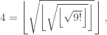
 Conjecture: Suppose
  and
and  are given. Then using the factorial function and the function
 and
and  from
from  and so on, but you’ve got to get larger first, and that requires some use of the factorial.
 there exist positive integers
  such that
 is composed
  times.
 The Possibility Lemma is only a starting point, since it turns out that most of the time, the smallest
  need to generate a particular
  is actually greater than
  the smallest
  with
with  so that
 we get
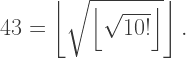

 is
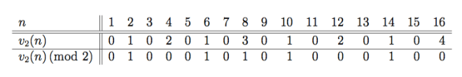
is  and computations with such large factorials take time. It turns out that the trick was to compute in advance the first 1,000,000 factorials as floating point numbers. A little accuracy is lost as result, but several checks suggested that even so, the correct value of
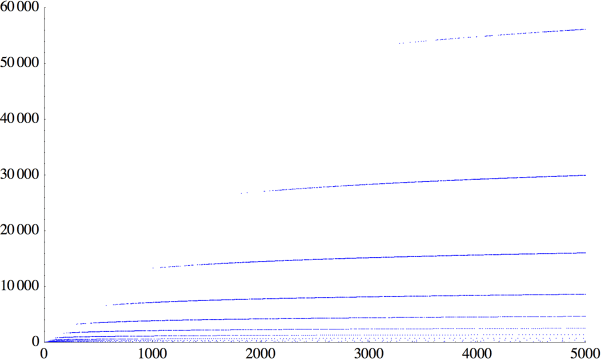
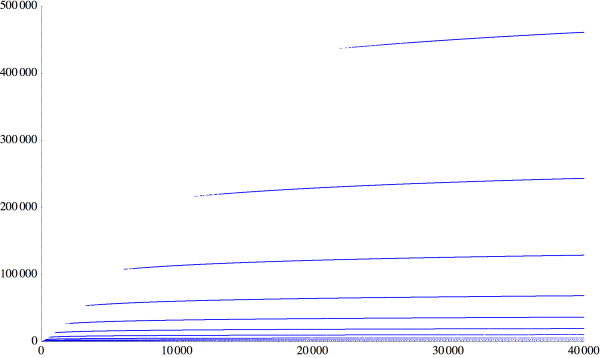
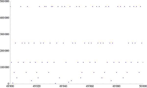
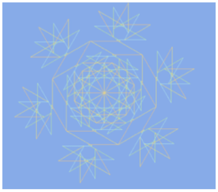
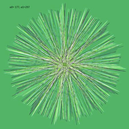
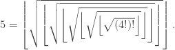
 generates the following graph, so it seems that there may be similar behavior for various
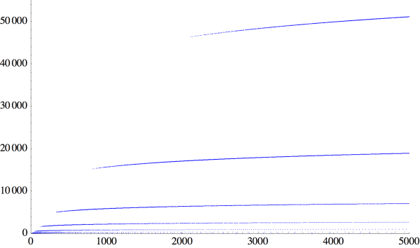
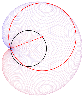
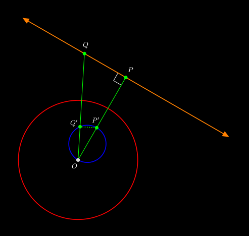
![[OP]\cdot[OP']=[OQ]\cdot[OQ']=1,](https://s0.wp.com/latex.php?latex=%5BOP%5D%5Ccdot%5BOP%27%5D%3D%5BOQ%5D%5Ccdot%5BOQ%27%5D%3D1%2C&bg=ffffff&fg=333333&s=0&c=20201002) and so
and so![\dfrac{[OP]}{[OQ]}=\dfrac{[OQ']}{[OP']}.](https://s0.wp.com/latex.php?latex=%5Cdfrac%7B%5BOP%5D%7D%7B%5BOQ%5D%7D%3D%5Cdfrac%7B%5BOQ%27%5D%7D%7B%5BOP%27%5D%7D.&bg=ffffff&fg=333333&s=0&c=20201002)
 and
and  must have the same measure, making triangles
  and
and  similar triangles.
 is also a right angle. To summarize: given any point Q on the line, its inverse point Q′ has the property that when joined to O and P′, a right triangle is formed with a right angle at Q′.
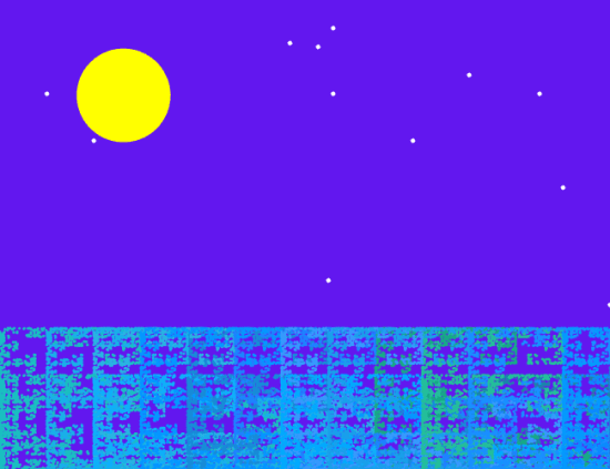
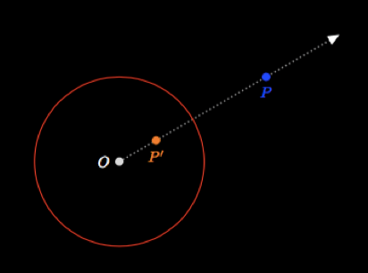
![[OP]\cdot[OP']=1,](https://s0.wp.com/latex.php?latex=%5BOP%5D%5Ccdot%5BOP%27%5D%3D1%2C&bg=ffffff&fg=333333&s=0&c=20201002)
![[AB]](https://s0.wp.com/latex.php?latex=%5BAB%5D&bg=ffffff&fg=333333&s=0&c=20201002) denotes the distance from A to B. That is, when you multiply the distances from the origin of a point and its inverse point, you get 1.
denotes the distance from A to B. That is, when you multiply the distances from the origin of a point and its inverse point, you get 1.
![[OO]\cdot[OO']=1.](https://s0.wp.com/latex.php?latex=%5BOO%5D%5Ccdot%5BOO%27%5D%3D1.&bg=ffffff&fg=333333&s=0&c=20201002)
 — it is often useful to add the number ∞, so that division by 0 is now possible. This results in the extended complex plane, and is very important in the study of complex analysis.