Digital Art VII: Final Projects!

It’s hard to believe that the semester has finally come to an end!  And I must say that Mathematics and Digital Art was one of most enjoyable courses I’ve ever taught.  I’ll summarize my thoughts in a later reflective post, but today I’d like to showcase my students’ Final Projects.  There really was some exceptional work — but I’ll let the images speak for themselves.

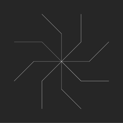
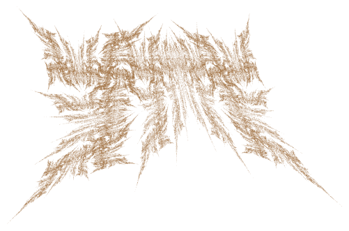
Many students built upon the work we did earlier in the semester. Safina used several different elements we explored during the course.  In addition, she researched turtle graphics in Python to incorporate additional elements (those with lines emanating from a central point).

SM-MathProjectFinal.png


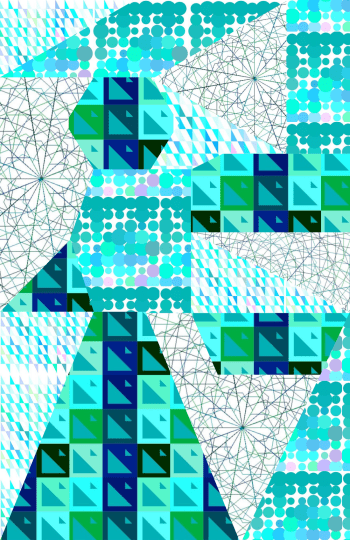
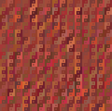
A few students especially enjoyed the work we did with color and Josef Albers, and created projects around different ways to contrast colors.  Andrew created many variations on a triangular theme.

screen-shot-2016-11-20-at-7-02-02-pm

He took this idea further, and went so far as to combine different triangles in composite images.

Hexagon-01.png

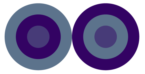
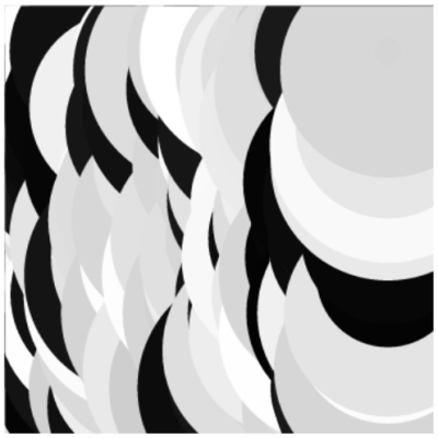
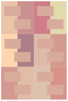
Julia, on the other hand, experimented with other geometrical objects.  She played with having colors interact with each other, and created the following image.  Although it may not look like it, the two center circles are in fact exactly the same color!

jn-capture7

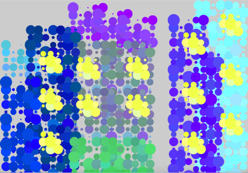
Two students were interested in image processing, and worked closely with Nick to learn how to use the appropriate Python libraries in order to work with uploaded images.  Madison’s work focused on sampling pixels in an image and replacing them with larger circles to create an impressionistic effect.  She found that using a gray background gave the best results.

MJ-Screen Shot 2016-11-30 at 9.51.23 PM.png


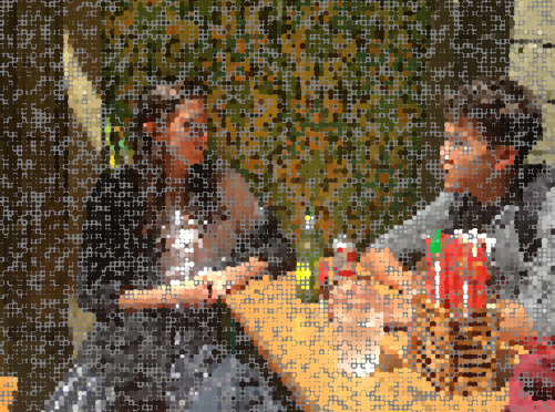
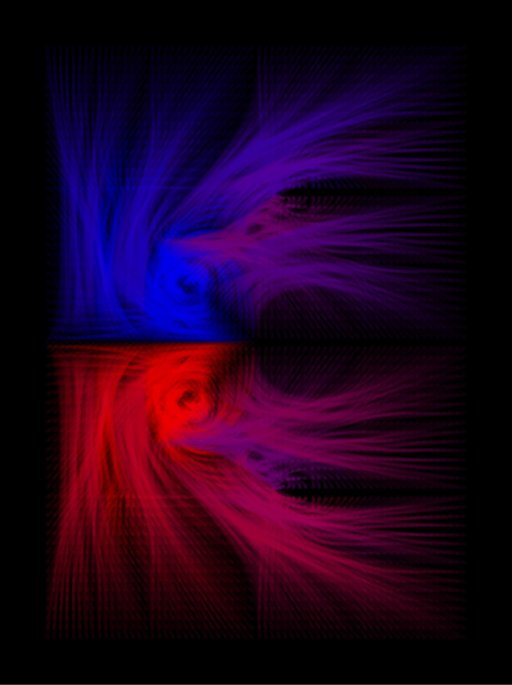
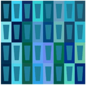
Lucas also worked with image processing.  He began by choosing a fairly limited color palette.  Then for each pixel in his image, he found the color on his palette “nearest” the color of that pixel (using the usual Euclidean distance on the RGB values), and then adjusted the brightness.  The image below is one example illustrating this approach.

LA-Screen Shot 2016-12-04 at 11.42.53 PM.png


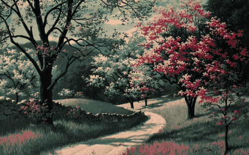
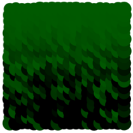
Two students worked with textures we experimented with earlier in the semester to create pieces like Evaporation.  Maddie wanted to recreate a skyline of Dubai (photo from the Creative Commons).

mc-dubaiskyline

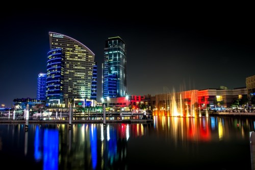
She picked out particular elements to emphasize in her work.  You can clearly see the tall buildings and lit windows in a screenshot of her movie.

MC-Screen Shot 2016-12-02 at 9.26.26 AM.png


Sharon was interested in working with some of Dali’s paintings, creating impressionistic images by mimicking Dali’s color palette.  Here is her interpretation of The Elephants.

sa-screen-shot-2016-12-11-at-1-28-20-pm

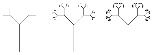
Although we only touched on L-systems briefly in class, Ella wanted to focus on them in her project.  Nick also worked closely with her to create different effects.  Here is a screenshot from one of her movies.

ek-screen-shot-2016-12-11-at-1-33-30-pm

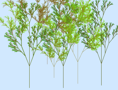
She was able to create some interesting effects by just slightly altering the parameters to L-systems which created trees and superimposing the new L-system on top of the original.  This gave some depth to the trees in her forest.

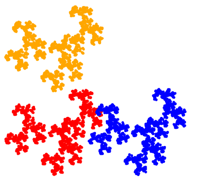
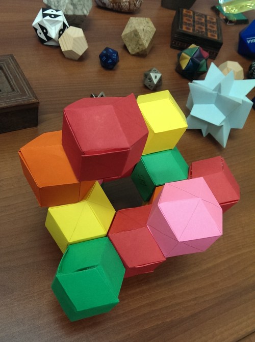
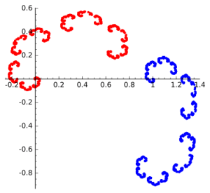
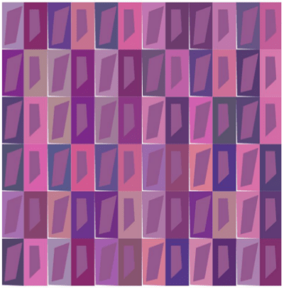
And one student decided to revisit Iterated Function Systems, but this time using nonlinear transformations in a variety of different ways.  Here is one of her images.

af-screen-shot-2016-12-04-at-7-51-12-pm
So you can see the wide range of projects students undertook!  This typically happens when you give students the freedom to choose their own direction.  I was also inspired by the enthusiasm of some of the students’ presentations.  They really got into their work.

The last assignment was to write a final Response Paper about the course.  The prompt was the same as that for the Response Paper I assigned midway through the course, so I’m curious to see if their attitudes have changed.  I’ll talk about what I learn in next week’s post!


Digital Art VI: End of Week 14

The last three weeks have been very intense!  The main focus has been on laboratory work, both with Processing and Final Projects.

Week 12 began with another round of Presentations on papers from past Bridges conferences.  This proved to be successful again — with topics ranging from geometrical furniture to zippergons to maps of Thomas More’s Utopia.  We all learned something new!

The time not spent on Presentations that week was devoted to working on projects.  Students were finding their stride, and their ideas were really beginning to take shape.

Two students were interested in image processing, so Nick has been working with them.  The initial problem was that doing anything in Sage involving image processing was just too slow — you’re code is essentially sent to a remote server, executed, and the results sent back.  Since we’re using the free version, this means performance is unpredictable and far too slow for computation-heavy tasks.

So Nick helped with installing Python, finding image processing packages, etc.  This process always takes a lot longer than you imagine, but eventually all issues were resolved.

While Nick was working on image processing, I was helping others.  One student was really interested in using L-systems — one of my favorite geometrical topics recently!   But all my work with Thomas involved code written in Postscript and Mathematica.  Which meant I had to rewrite it in Python.

This proved to be quite a bit trickier than I thought.  The student was looking at The Algorithmic Beauty of Plants, and was interested in modeling increasingly complex L-systems.  First, the simplest type, like that used to generate the Koch curve.  Next came bracketed L-systems, and then bracketed L-systems with multiple rules.  I did finally get all these to work; I intend to clean up the code and share it in a future post.

Week 13 was devoted entirely to Processing and project work.  I started the week with introducing a few new ideas.  What really inspired the class were the mouseX and the mouseY variables.  When your mouse is in screen space, the mouseX and mouseY variables contain the location of your mouse.  So you can put an object where the mouse is, or have the x-coordinate of the mouse in some way determine the color or the size of the object.  The possibilities are virtually endless.

Here’s a sample movie made with this technique.

Since the code is just a few lines long, it won’t take long to explain.  Here is the complete program:

mouseanddot

The drawPoint function will draw a point centered at the position of the mouse.  But in addition to those coordinates, the function takes an addition argument:  float(mouseX)/500.  This argument is 0 at the left edge of the screen, and 1 at the right edge.  (Recall the need for “float,” since otherwise Python will perform integer division and give 0 for any number less than 500.)

So the stroke command uses the parameter p to determine how much red is in the color specification.  When p is 0, there is no red, so the dot is black.  And when p is 1, the dot is red.  I used “p**0.4” as an illustration that interpolation need not be linear — the exponent of p determines how quickly or slowly the dot gets brighter as you move the mouse to the right.  Of course the dot also gets larger as you move your mouse to the right, as is clear by the strokeWeight function call.

I showed this example as I introduced the movie project.  Their assignment was to make a movie — anything they wanted to try.  The complete prompt is given on Day 34 of the course website, but I’ll give the gist of it here.  The main goal was to have students use linear interpolation in at least four different ways in their movie.  Of course they could use nonlinear interpolation if they wanted to, but it wasn’t required.

There was no length requirement — it’s easy to make a movie longer by adding more frames.  Just be creative!  Interpolation is a very useful tool in making movies and animations, and has a mathematical basis as well.  So I wanted that to be the focus of the project.  I also had them write a brief narrative about their use of interpolation.

This is Andrew’s movie.  You can clearly see the use of interpolation here in different ways.  It was also nice to see the use of trigonometry to calculate the centers of the dots.


Ella was interested in L-systems, and so Nick spent some time working with her on Python code during his weekly office hours.  Here is what she created.


Lucas wanted to use some interaction with the mouse, and he also had the idea of the sun setting as you moved the mouse down the screen.  Watch how the fractal clouds move with the location of the mouse as well.


So you can see how varied the use of interpolation was!  The students really enjoyed having control over the possible special effects, and created a wide range of interesting features in their movies.

That takes us to Week 14.  On Monday, we had a guest speaker come in, Chamberlain Fong.  I met him in Finland at Bridges this summer, only to find out he lives the next neighborhood over in San Francisco!  He gave a very interesting talk about taking pictures with a spherical or hemispherical camera lens, and the issues involved in printing the pictures.

The problem is essentially the same as creating a map of the globe — making a sphere flat.  There will always be distortion, but you have some control over what type of distortion.  You can keep angles the same, or areas the same — or some combination of the two.  And as these cameras keep getting cheaper, there will be a growing interest in making your spherical photos look realistic.

And although we had class on Wednesday, some students had already left for Thanksgiving Break.  So Nick and I were available to help on an open lab day.  Most of the students actually showed up, and we had a productive day working on movies (which were due Wednesday) and projects.

The next (and final!) post on Mathematics and Digital Art will survey the students’ Final Projects, so stay tuned!

Digital Art V: End of Week 11

It’s been an exciting three weeks in Mathematics and Digital Art!  We began Week 9 after our Fall break with a talk by Carlo Sequin.  Here’s Carlo with one of his sculptures at the University of California, Berkeley.

imag3969

I met Carlo through the Bridges conferences; he currently sits on the Board.  Since he’s so close by, I thought it would be great to have him visit my class.

His talk centered around the computer graphics programs he wrote in order to design sculptures like the one you see in the picture above.  Carlo included several different parameters, allowing an incredible variety of images to be generated.

Then he focused on a few of his sculptures and described the design process from conception to final sculpture.  He even remarked how he got lucky once — he and his team forgot to measure the width of the door they needed to take the sculpture through, and it fit with just a few inches to spare….

Friday, Day 24, was our first Project day.  Students’ ideas were still somewhat vague — they did have to write a Proposal, but still didn’t have a clear direction.  We made some progress, though the next Project day helped quite a bit more.

On Monday, Day 25, we dived into working with Processing.  I kept in mind the comments from students’ response papers which I mentioned in my previous post — they really wanted to learn more about code.

Now coding is a precision endeavor, as there is no room for error as far as syntax is concerned.  So after working through a simple example, I presented them with the following movie.

Admittedly it’s not a blockbuster…but their lab work was to duplicate this movie as precisely as possible.  I gave them a basic template (see the May 2016 archives for the start of a six-part series on Processing which I used as a basis for their lab work), but they didn’t just have to tweak numbers — they also had to add new elements.

The main mathematical tool involved was linear interpolation, which we went over in some detail in class.  The next class, I had them work on recreating the following movie.

This proved a bit more challenging.  Some students at first thought there was a rotation involved — but it’s just linear interpolation again, on a somewhat larger scale.  Here are the prompts I gave them:

  • the screen is 500 x 500 pixels;
  • the dots are always 25 pixels from the edge;
  • the colors are the standard red, green, blue, and orange;
  • the smaller dots are 100 pixels wide, and the larger ones are 200 pixels wide.

The main challenge was working in screen space, since they needed to calculate the exact centers of the circles.  Of course students progressed at different rates, and they were finally getting the main point — you can use linear interpolation to morph any aspect of an image which depends on a numerical parameter.  As a mathematician, I was used to thinking along these lines all the time, but it’s a concept that takes a while to really sink in if it’s new.

Friday, Day 27, was our next project day.  We worked at fleshing out more details of the students’ various projects.  Two students wanted to explore image processing, so Nick continued working with them to download the appropriate packages and get Python installed on their computers.  Such projects are never as easy as they sound, but Nick did get everything to work.

While he was doing that, I circulated with the other studets, discussing their projects and answering a few questions about making movies, if they had them.  It was a productive day, and everyone left class with a much clearer idea of their project than they had the week before.

On Monday, we continued our work with Processing.  I went through an example from my earlier blog posts — making a movie which morphs a Sierpinski triangle — in some detail, explaining it line by line.  Again, the most challenging part was converting from user space to screen space.  A fractal which fit in a unit square had to be scaled and moved to fit nicely into screen space.

This took just about the entire class.  Although we had done work previously with iterated function systems, we did have to take some time to review certain aspects of the code we used before.  Then on Day 29, I had them duplicate the following movie.

In order to focus on the coding, I began the movie with a fractal they had on a previous quiz, so they knew which affine transformations to start with.  They had to figure out how to modify one of the transformations to produce the final image, and then use linear interpolation to create the movie.

This proved challenging, but everyone made good progress during the lab.  They are supposed to finish by Monday.

On Friday of Week 11, we had our second guest speaker — Shirley Yap from California State University, East Bay.  I met Shirley last February when Nick and I went to a regional meeting of the Mathematical Association of America.  She was in charge of organizing the Art Exhibition Nick and I had pieces in.

After showing a few interactive examples from her web page, Shirley focused her discussion on the following piece she created.

glassleaves_0
Leaves of Glass

She talked a lot about the challenges of making a physical piece, rather than a work of digital art.  For example, she actually wanted to use glass, but is was not possible to etch in glass given the tools she had available.  So she had to settle for acrylic, which is very easy to smudge if you aren’t careful.  You see, the individual squares can pivot where they are screwed in, so the artwork is interactive.

There were also size requirements, since she had to be able to take in on the airplane with her to a conference.  Other issues arose — in some ways working digitally is a lot easier.  As Shirley remarked, once you drill a hole, you can’t undrill it…but it’s easy to change a parameter in digital work.

What was really nice was that Shirley talked about mathematical envelopes (one of my favorite topics; I’ve written about it before on my blog), and the curves she used to make her envelopes — Bernstein polynomials.  She took the time to go through a few simple examples, so that students got a sense of what these curves are like.  It was a nice example of yet another topic in mathematics students hadn’t seen before being used to create art.  Truly, mathematics is everywhere….

Stay tuned for the next update of Mathematics and Digital Art!

Digital Art IV: End of Week 8

The last two weeks were focused on a study of polyhedra.  While not strictly a digital art topic, I thought it important for students to develop a basic three-dimensional vocabulary in the event they wanted to do further study in computer graphics.

imag4281

We began with the Platonic solids, naturally, looking at enumerating them geometrically and algebraically.  The algebraic enumeration involved solving the usual

\dfrac1p+\dfrac1q=\dfrac12+\dfrac1E.

This proved challenging, especially when I gave some additional, similar Diophantine equations for homework.  We also took time to build a dodecahedron and an icosahedron.  This occupied us on Day 17, Day 18, and part of Day 19.

Since the first half of the semester was nearing its end, it was time to begin thinking about Final Projects.  So I took the rest of Day 19 to help students individually choose a topic, and assigned the Project Proposal over the weekend.

We had a brief discussion of graph theory on Day 20, which involved looking at the adjacency graphs of the vertices of the Platonic solids, such as the one for the dodecahedron.

graphdodeca

I introduced much of the basic vocabulary, using the chapter I wrote in my polyhedra textbook as a guide.  Of course there is only so much progress to be made during a single class, but I did want to indicate how two apparently different areas in mathematics are related.

The homework involved untangling adjacency graphs, such as the one below.

graphprism

This is just a triangular prism, although drawn a little unconventionally.  This assignment again proved more difficult than I thought, even with Euler’s formula to help in calculating the number of faces.  So we spent extra time on Day 21 going over the homework, followed by a very brief discussion of duality.  And as students were having difficulty narrowing their focus for their project proposals, I spend the rest of Day 21 talking individually with them as they started building a few rhombic dodecahedra.

Over half of Day 22 was taken up by a quiz on their homework; I didn’t want there to be much time pressure.  The last part of this class was spent creating an in-class sculpture with rhombic dodecahedra.  I chose this dual model for them to build as it is space-filling.

I was surprised at how much they really got into it!  I do hope we have time for a similar project at the end of the semester.  We were in a bit of a rush for time, but still managed to create something intriguing.

imag4318

Last time I mentioned I assigned a short response paper getting feedback from the students about how the course was going so far, and I said I’d share some of their comments.  All (anonymous) quotes are from student papers.

I really like how hands-on the course is, and how there is a good balance between lecture and lab time.

This was a common opinion — and validates a major feature of the course design.  I am glad students appreciate it!  Another student made a similar remark about the lab time.

I enjoy the lab assignments that we get because I like the designs I create.  It allows us to put to practice what we have learned with each lesson.

I specifically asked about how students’ attitudes about mathematics changed.  I got some encouraging responses.

I was used to thinking of math as just something I had to do, that would probably be useful later in life, but wouldn’t really pertain to whatever I wanted to do with art.  I’ve realized that I would actually really like to use this kind of math in my art in the future, because I never realized what kind of things I could make with this medium.

As someone who wasn’t the best at geometry in high school (I’m more of an algebra person), I think this class has given me a practical use for all the things I learned in high school that I found difficult to grasp or uninteresting.

I was pleased to read responses like this, since again, this reflects an overarching purpose of the course — see how mathematics can actually be used in practice.  One student even went so far as to say,

I would also like to mention something, though this might not be considered significant, I never thought I would have to use matrices ever again in my life.

A few students remarked on using mathematics in the creative process.

At first, I was a little unsure of the role that mathematics took in graphic design, but as soon as we started playing with Sage, I noticed that it affects almost every aspect brought forth in the image.

Making “rules” for you art was something very different for me…..combining the left brain and the right brain creates incredible pieces of work….

Some students made more specific comments.  One student liked the presentations the best.

Looking through the different papers in the Bridges archive and hearing everyone’s presentations really made me realize the extent that mathematics is related to so many other topics.

In addition, I asked for specific suggestions for improvement.  By far the most common remark was that students want to learn more about how the Python code in Sage works.  I was really encouraged when I read those comments!  We will start to learn Processing in a few weeks, and I’ll make sure we discuss the code in more detail.

One student really liked the discussion board I set up for a few of the assignments — it is not difficult to create discussion boards for future assignments, so we’ll try that again.  Another remarked that it would be good to learn about the printing process — and I certainly agree!  But as I remarked in previous posts, I thought the logistics of this challenging endeavor would be too difficult to implement.  It is certainly a future goal.

But overall, I was very glad to read how students were enjoying the course — and also pleased about their suggestions for improvement.  So I’ll work hard at making the second half of the course even better than the first!

Koch Curves and Canopies

Time for another “math in the moment” post!  There have been a few interesting developments just this past week, so I thought I’d share them with you.

The first revolves around the Koch curve.  I’ve talked a lot about the algorithm used to generate the Koch curve when the angles are changed — but this is the first time I’ve experimented with three different angles.  For example, the recursive procedure

F   +45   F   +180   F   +315   F

generates the following spiral:

spiral8

Looks simple, right?  Just 16 line segments.  But here’s the unexpected part — it takes 21,846 iterations to make!  That’s right — the horizontal segment in the upper left is the 21,846th segment to be drawn.

Why might this be?  Partly because of the fact that one angle is 180, and also the fact that 45 + 415 = 360.  In other words, you are often just turning around and retracing your steps.  These arms are retraced multiple times, not just once or twice like in previous explorations.

I found this family of spirals by having Mathematica generate random angles and using the algorithm to draw the curves.  Without going into too many details, the “obvious” way to generalize the equation I came up with before didn’t work, so I resorted to trial and error — which is easy to do when the computer does all the work!

Notice the pattern in the angles:  45 (1/8 of a circle), 180 (1/2 of a circle), and 315 (7/8 of a circle).  Moving up to tenths, we get angles of 36 (1/10 of a circle), 180 (1/2 of a circle), and 324 (9/10 of a circle), which produce the image below.

spiral5.png

Notice there are only five arms this time (not 10).  And it only takes 342 segments to draw!  There’s an alternating pattern here.  Moving up to twelfths gives 12 arms, and takes a staggering 5,592,406 segments to draw.  Yes, it really does take almost 6,000,000 iterations to draw the 24th and last segment!

With the help of Mathematica, though, I did find explicit formulas to calculate exactly how many iterations it will take to draw each type of image, depending on whether there are an even number of arms, or an odd number.  Now the hard part — prove mathematically why the formulas work!  That’s the next step.

I hope this “simple” example illustrates how much more challenging working with three different angles will be.  I think working out the proof in these cases will give me more insight into how the algorithm with three angles works in general, and might help me derive an equation analogous to the case when the first and third angles are the same.

The second development is part of an ongoing project with Nick to write a paper for the Bridges 2017 conference in Waterloo.  The project revolves around fractal trees generated by L-systems.  (We won’t be discussing L-systems in general, but I mention them because the Wikipedia had a decent article on L-systems.)

trees1

Consider the examples above.  You first need to specify an angle, a, and a ratio, r.  In this example, a is 45 degrees, and r is 0.5.  Start off by drawing a segment of some arbitrary length (in this case the trunk of a tree).  Then turn left by the angle a, and recurse using the length scaled by a factor of r.  When this is done, do the same recursion after turning right by the angle a.

On the left, you should see three different sized lengths, each half the size of the one before.  You should also be able to easily see the branching to the left and right by 45 degrees, and how this is done at each level.

In the middle, there are six levels, with the smallest branches only 1/32 the length of the tree trunk.  Can you guess how many levels on the right?  There are twelve, actually.  At some point, the resolution of the screen is such that recursing to deeper levels doesn’t actually make the fractal look any different.

What Nick is interested in is the following question.  Given an angle a, what is the ratio r such that all the branches of the tree just touch?  In the example below with a being 45 degrees, the leaves are just touching — increasing the ratio r would make them start to overlap.

trees2

What is r?  It turns out that there’s quite a bit of trigonometry involved to find the precise r given an angle a, but it’s not really necessary to go into all those details.  It’s just enough to know that Nick was able to work it out.

But what Nick is really interested in is just the canopies of these trees — in other words, just the outermost leaves, without the trunk or any of the branches.

canopy1

Right now, he’s experimenting with creating movies which show the canopies changing as the angle changes — sometimes the ratio is fixed, other times it’s changing, too.

Two observations are worth making.  First, this was a real team effort!  Nick had done the programming and set up quite a bit of the math, and with the aid of Mathematica, I was able to help verify conjectures and get the expressions into a useable form.  We each had our own expertise, and so were each able to contribute in our own way to solving the problem.

Second, Nick is using mathematics to aid in the design process.  My first attempts to create symmetric curves using the algorithm for the Koch snowflake were fairly random.  But now that I’ve worked out the mathematics of what’s going on, I can design images with various interesting properties.

Likewise, Nick has in mind a very particular animation for his movies — using the just-touching canopies — and is using mathematics in a significant way to facilitate the design process.  Sure, you can let the computer crunch numbers until you get a good enough approximation — but the formula we derived gives the exact ratio needed for a given angle.  This is truly mathematical art.

I’ll keep you updated as more progress is made on these projects.  I’ll end with my favorite image of the week.  The idea came from Nick, but I added my own spin.  It’s actually canopies from many different trees, all superimposed on each other.  Enjoy!

canopy2

Digital Art III: End of Week 6

Recall that at the end of Week 4, we had just begun a lab on affine transformations and iterated function systems.  At the beginning of Week 5 (Day 11), students were supposed to finish the exercise they began on Friday, and try another.  This was the new prompt:  Create a fractal using two affine transformations. For the first, rotate by 60 degrees, then scale the x by 0.6 and the y by 0.5. For the second transformation, rotate 60 degrees clockwise, scale the x by 0.5 and the y by 0.6, and then move to the right 1.  I provided a link to the fractal which should be produced, shown below.

d11fractal

Again, this proved to be a challenge!  The reason is that the computer is somewhat unforgiving.  To produce the image above, every calculation has to be correct.  Here were some common issues:

  1. There was difficulty interpreting the statements as geometric transformations.  In particular, getting the order of the matrix multiplication correct, and interpreting a clockwise rotation as a rotation by -60 degrees.
  2. Performing the matrix multiplication correctly.  Some students were using online calculators, and some had trouble with converting degrees to radians.
  3. Translating the results into Python code; the affine transformations needed to be converted to the form (ax+cy+e, bx+dy+f).

I also gave them an exercise to reproduce one of the fractals they needed to analyze for homework the previous week.

This occupied us for all of Week 5, since I also wanted to give them time to work on their upcoming assignment.

Week 6 was our first Presentation Week.  Since we’d only need two days for the presentations given the class size, I spent the first day of the week giving my Bridges talk on producing Koch-like fractal images.

The class was interested to learn more about this algorithm, and I had hoped to spend a week devoted to the topic.  But because of the Processing work we’ll be doing later — animation of fractals using iterated function systems — I didn’t want to rush through the preliminary work on affine transformations and IFS.  Any misunderstandings now would surely be problematic later.

The presentations were to be on papers from the Bridges archives.  All papers since the Bridges conferences began (which was in 1998) are archived online.  The assignment was simple:  find a paper in the archive that’s at least four pages long, and give a five-minute presentation on it to the class.  I did create a discussion board where they posted the title/author of their selections so there wouldn’t be any duplicate presentations.

These presentations went very well.  Most students’ presentations were close to ten minutes long, and the enthusiasm for their presentations was quite evident.  I must admit that I learned a lot, too — I had not read most of the papers they selected.

I had students do simple peer evaluations, and included the item “I would like to learn more about this topic after hearing the presentation.”  They selected a number from 1–5, with 5 meaning “most interested.”  The overall average score was about 3.9 — meaning the papers piqued their curiosity.  In addition, I wanted to get additional ideas about what to include in the few days I set aside for special topics at the end of the semester, or what new ideas to incorporate into next semester’s class.

The most popular paper (4.75 average) was On Generating Dot Paintings in the Style of Howard Arkley, which Madison said reminded her of some of the textures we created during a few of our lab sessions.  The next highest average was 4.25, so this was the clear favorite.  I hope we’ll have time to explore it further later on.

And that took us to the end of Week 6!  I had hoped to have some time in the lab to have students find interesting polyhedra nets they’d like to build, since the next two weeks will be devoted to polyhedra.  No, it’s not really a digital art topic — but it is an area of expertise.  I wanted students to have some exposure to three-dimensional geometry since if they continue to study computer graphics, they will certainly move from two into three dimensions.

Now it’s time to look at some student work!   I’ll focus on one fractal from the assignment on iterated functions systems.  Here is the prompt:  Create a morphed Sierpinski triangle, based on the code in the Sage worksheet. The idea is to have your fractal look like it was derived from a Sierpinski triangle, but just barely. Someone looking at it should wonder about it, and maybe after 30 seconds or so, say “Hey, that looks like a Sierpinski triangle!”

One student created the following image, and wrote:

I think this fractal looks like many sets of pine trees, and I like the way that it shears out. I made the whole thing the same color (gray) to make the fact that it was derived from the Sierpinski triangle less obvious.

af2

Julia creating the following fractal image, and remarked that at one point, she went “too far” and had to backtrack a bit.

jn3

Safina went a different direction, and created this.

sm4

She wrote,

The stretch and rotation reminds me of a tree, more specifically a Christmas tree….I wanted to emulate a sort of Christmas feel because I was listening to Christmas music.

So motivation can come from anywhere!  I’ll post more of their images on my Twitter feed, @cre8math.

Again, you can see how my students are really embracing the course and being very creative with the assignments.  I’m looking forward to seeing more of their work.

I just assigned a brief response paper asking students how they felt about the course so far, and how it has changed their ideas about art, mathematics, and computer science.  I’ll report on their comments in my next summary in two weeks.  Stay tuned!

Digital Art II: End of Week 4

It’s hard to believe it’s been four weeks already!  Recall that we ended Week 2 with work on an Evaporation piece.  We’ll see examples of student work after a brief recap of Weeks 3 and 4 (Days 6–10).

In the past two weeks, we focused on affine transformations and their use in creating fractals with iterated function systems.  This was not intended to be a deep discussion of linear algebra, but a practical one — how affine transformations reflect the geomtetry of fractal images.

Beetle2
Fractal beetle created with an iterated function system.

Days 6 and 7 were an introduction to the geometry of affine transformations.  I like to emphasize the geometry first, so I worked to find a way to simply and unambiguously describe an affine transformation geometrically.

affinetransformation

The blue square represents the unit square, and the red parallelogram the transformed square.  The filled-in/open black circles on the parallelogram represent how (0,0) and (1,0) are transformed, respectively.  Additionally, the pink fill in the parallelogram represents that fact that there is a flip (that is, the determinant of the linear part of the transformation is negative).  Strictly speaking, this coloring isn’t necessary, but I think it helps.

We then worked on writing the affine transformation in the form

T\left(\begin{matrix}x\\y\end{matrix}\right)=\left[\begin{matrix}a&b\\c&d\end{matrix}\right]\left(\begin{matrix}x\\y\end{matrix}\right)+\left(\begin{matrix}e\\f\end{matrix}\right)

We did this in the usual way, where the columns of the matrix represent where the unit basis vectors are transformed, and the vector added at the end is the translation from the origin.  These can all be read from the diagram, so that the picture above describes the affine transformation

T\left(\begin{matrix}x\\y\end{matrix}\right)=\left[\begin{matrix}-2&-3\\2&0\end{matrix}\right]\left(\begin{matrix}x\\y\end{matrix}\right)+\left(\begin{matrix}-2\\1\end{matrix}\right).

To help in visualizing this in general, I also wrote a Sage worksheet which produces diagrams like the above picture given the parameters af.  In addition, I showed how the vertices of the parallelogram may be found algebraically by using the transformation itself, so this meant we could look at affine transformations geometrically and algebraically, as well as with the Sage worksheet.   (Recall that all worksheets/assignments may be found on the corresponding day on the course website.  In addition, I have included the LaTeX code for the assignments for those interested.)
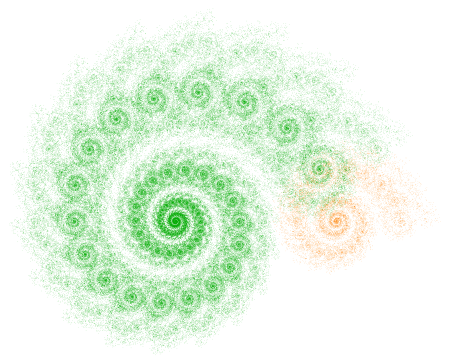
I explained several different types of affine transformations — translations, reflections, scalings, and shears.  On Day 8, we saw how to write the affine transformations which describe the Sierpinski triangle, and students got to play with creating their own fractals using the accompanying Sage worksheet.

On Day 9, I took about half the class to go through three of my blog posts on iterated function systems.  I emphasized the first spiral fractal discussed on Day035, paying particular attention to the rotation involved and matrix multiplication.

Two2

Most students weren’t familiar with trigonometry (recall the course has no prerequisites), so I just told them the formula for rotation matrices.  We briefly discussed matrix multiplication as function composition.  I gave them homework which involved some practice with the algebra of matrix multiplication.

On Day 10, we began with going over some previous homework, and then looked at what transformations were needed to producing the fractal below (as practice for their upcoming homework).

revsierpinski4

We then engaged in the following laboratory exercise:  Create a fractal using two affine transformations.  For the first, rotate by 45 degrees, then scale the x by 0.6 and the y by 0.4, and finally move to the right 1.  For the second transformation, rotate 90 degrees clockwise, and then move up 1.

This was practice in going from a geometrical description to a fractal — they needed to perform the appropriate calculations, and then enter the data in the Sage worksheet and see if their fractal was correct (I gave them a link to the final image).

This turned out to be very challenging, as they were just getting familiar with rotations and matrix multiplication.  So we’ll need to finish during the next class.  I’ll also give them another similar lab exercise during the next class to make sure they’ve got it.

Last week’s digital art assignment was another success!  Again, I was very pleased with how creative my students were.  If you look back at the Sage worksheets, you’ll see that the class was working with color, texture, and color gradients (like my Evaporation piece).

One student created a texture with a lot of movement by keeping the circles separate and using a wide range of gray tones.

af_1

Maddie took advantage of the fact that the algorithm draws the circles in a particular order to create a scalloped texture.  This happens when the circles are particularly large, since the circles are drawn in a linear fashion, creating successive overlap.

mc_2

Another student also used this overlapping feature with a color gradient.  He describes his piece as follows:

This piece is what I like to call “The Hedge” as it reminds me a lot of those tall square hedges that are in mansions. It’s as if the light is hitting the top of the hedge and dispersing down into the shadows and thickness of the leaves. I especially like the leafy effect the overlapping circles give.

la_1

Finally, Madison experimented with altering the dimensions of the grid to create a different feel.

mj_1

She thought that making the image wider made the evaporation effect more pronounced.

These are just some examples of how students in my Mathematics and Digital Art course take ideas I give them and make them their own.  They are always asking how they can incorporate one effect or another into their work, and Nick and I are glad to oblige by helping out with a little code.

As I strive to keep my posts a consistent length, I won’t be able to share all the images I’d like to this week.  So I’ll be posting additional images on my Twitter feed, @cre8math.  Follow along if you’d like to see more!

Digital Art I: End of Week 2

Mathematics and Digital Art is well underway!  As promised, I’ll be giving weekly or biweekly summaries of how things are going.  You’re also welcome to follow along on the course website.

Day 1 was the usual introductory class, with a discussion about the syllabus and what the course would be like.  (Remember I blogged a four-part series on the course beginning at Day045.)  I wanted to make it clear that there would be both mathematics and coding in the course.  Some students ended up dropping the course the first week as a result, leaving the class with nine students.

On Day 2, I discussed representing color on the computer — using RGB values (both integer and real), as well as using hexadecimal notation.  Since the course has no prerequisites, we really did need to start at the beginning.  Students did some exploring with various RGB values using a Sage worksheet.  (Links to all the worksheets and other websites referenced in class can be found on the course website.)

Josef Albers was the topic of Day 3.  I’ve talked a lot about his work before, so I won’t go into great detail here.  I let students try out a Sage worksheet — they had an assignment to create their own version which was due in about week, so we spent half the class starting the project.

Day002Albers6Web3

Essentially, they needed to choose a color scheme and size for their piece.  But then they needed to use five different random number seeds, and decide which of the five resulting images looked best to them, and why.  So the assignment included a brief narrative as well.  The complete prompt is on my website.  (And I think I’ll just stop saying this — just know that anything I mention in these posts will be discussed in more detail on the course website.)

The next two classes focused on creating a piece based on Evaporation.

Day011Evaporation2bWeb

Again, I discussed this in some detail before (Day011 and Day012).  The basic idea is to use randomness to create texture, both with color and geometry.  Add to this the idea of a color gradient, and that’s enough to get started.

I took a bit of time on Day 5 to explain in some detail about how to create color gradients using a function like y=x^p, where p>0 — it isn’t exactly obvious if you’ve never done it before.  Having Nick as my TA in the class really helped out — I was at the board, and he was at the computer drawing graphs of functions and varying the parameters in the routine to produce color gradients. We worked well together.

It turns out that having two of us in the computer lab is really great — debugging takes time.  Students are gradually getting accustomed to the Sage environment, and  learning to go back and redefine functions if they get an error message indicating that something is undefined….

I have really been enjoying the laboratory experience!  My students are wonderfully creative, taking the basic motifs in directions I hadn’t considered.  I’ll illustrate with a few examples from the first assignment.  In this post and future posts, all work is presented with the permisson of the student, including the use of his/her name if applicable.

I should also remark that my intent is not merely to post pieces I subjectively like.  True to the title of my blog, Creativity in Mathematics, I intend to illustrate creative, original ideas.  I may feel that some students have been more successful with their ideas than others — but I’ll share that with the students individually rather than discuss it here.

In order to talk about the students’ creativity, however, let me show you the image they started with.sample

Andrew experimented with minimalism, creating a series of 2 x 2 images.  This is the one he said he liked the best because of the symmetry and contrast.

AQ_1

Julia was interested in exploring different geometries and created a few drafts which deviated from the rectangle-within-rectangle motif.  Here is one of them.

JN_1

Safina took a slightly different approach.  She wanted to create some variation by using trapezoids in the centers of the larger rectangles.

SM_1

Ella really worked with the geometry, creating a lot of visual contrast — especially with the asymmetrical polygons.

EK_1

So we’re off to a great beginning!  Right now, Nick and I are having to help a lot with editing code since it’s a new experience for most students.  But they are eager to learn, and as you can see, willing to explore new ideas, going well beyond where they started.  We can look forward to a lot more interesting work as the semester progresses!

P.S.  If you are ever interested in any of the students’ work and would like to discuss it further, send an email to vjmatsko@usfca.edu and I’ll forward it on to them!

Bridges: Mathematics and Art II

As I mentioned in my first post about Bridges 2016 (see Day038), one of my students, Nick, had artwork and a short paper accepted, and also received a $1000 travel scholarship! This week, I’d like to share his work with you. His paper is called Polygon Spirals. Here is the abstract (all quotes are taken directly from Nick’s paper):

Logarithmic spirals may be classically constructed with a chain of similar triangles that share the same center of similitude. We extend this construction to chains of n-
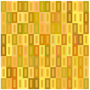
gons with centers on a logarithmic spiral with turning angle \pi/n, and scale factors with interesting properties. Finally, polygon spirals of this kind are used to produce a variety of artistic images.

I first learned of Nick’s interest in this type of spiral when he was in my Calculus II class, where he introduced a similar idea for his Original Problem assignment (see Day013). I encouraged him to continue with this project and submit his work to Bridges 2016. Here is Nick’s motivation in his own words:

The investigation of polygon spirals began by studying curves that arise when regular polygons with an odd number of sides are strung together. When polygons are strung together into a band by gluing them together along their sides, then the choice of what subsequent edge pairs are being used will define a turning angle introduced at each joint. In this paper we focus on bands made with minimal turning angles and with a consistent turning direction. Each odd n-gon defines its own turning angle, \pi / n. Moreover, by introducing a constant scale factor that modifies each subsequent polygon, a large variety of logarithmic spirals can be generated.

logarithmicpentagons
Figure 1: Logarithmic construction on pentagons
nestingarms
Figure 2: Spirals in phase

My original inspiration came from observing spirals of opposite handedness emerging from adjacent faces of the same polygon. The natural question that arose was which ratio to pick so that the two polygon chains would fall in phase, as in Figure 2. In other words, I needed to find the ratio such that every crossing point of the two logarithmic spirals coincided with the center of a polygon along each band. In this case, the two bands would share a polygon every period. I found this to be achieved when the golden ratio was applied to pentagons, which spurred a determination of the analogous ratio for generalized n-gons that corresponds to the sharing of every n^{\rm th} polygon. The construction hinges on similar triangles whose vertices are the center of a polygon, the center of one of that polygon’s children, and the center of similitude.

spiral
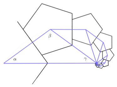
Figure 3: Logarithmic similar triangles

Referring to Figure3 (illustrated in the case n=5), \alpha=\pi/n and \beta=3\pi/n, so that \gamma=\pi/n. Now the triangle with angles labelled \alpha, \beta, and \gamma is isosceles because \alpha = \gamma. Moreover, the ratio between the longer and shorter sides is the same for all triangles since the spiral is logarithmic. If the shorter sides are of unit length, half of the base is \cos (\pi/n), making the base, and thus the ratio, equal to 2\cos (\pi/n).

Once the ratio has been found, spirals can be nested by applying a rotation of \pi/n. Completing this process yields n nested n-gon spirals.

With the ratio found above, it is not hard to show that the equation for one of the logarithmic spirals with this ratio, passing through the centers of the n-gons, has the equation:

r = (2\cos (\pi/n)) ^{n \theta/{\pi}}.

heptagons
Figure 4: Heptagon spiral

With most Bridges papers, there is a mix of mathematics and art. In fact, the first criterion listed on the Bridges website for art submissions is “Math content (this is a mathematically sophisticated audience.)” The second is “Esthetic appeal,” so artistry is important, too. What follows is Nick’s discussion of how he used the mathematical ideas discussed above to create digital art.

art3
Figure 5: Pentagon arms

Begin with a base polygon, and consider producing spirals from every face at every iteration. Although this would create too dense a pattern, it is possible to produce an interesting subset of this set of polygons using a random algorithm. This algorithm assigns a probability that a spiral is generated from each face of the n-gon, and this probability is randomly altered and then inherited by each child. The colors are also inherited and altered every generation. In Figure 5, the detailed texture is actually built of many small pentagons at a deep iteration. Off to the right can be seen a randomly generated pair of pentagonal arms falling into phase.

art1
Figure 6: Nested pentagon tiling

Figure 6 is a tiling of pentagons that features nested rings of pentagons with the property that any two adjacent pentagons differ in size by a ratio of the golden ratio. Figure 7 is an overlay of nonagon spirals with ratios between 0 and 1. This image captures the vast breadth of possible spirals based on a given n-gon, and the fascinating way that they interact.

art2
Figure 7: Nonagon spiral overlay

Figure 8 was randomly generated by the same algorithm which produced Figure 5, however with nonagons rather than pentagons. This picture illustrates the infinite detail of a fractal set based on interacting nonagon spirals.

art4
Figure 8: Nonagon bush

Quite an amazing sequence of images! Nick took a Python programming class his first semester, and so was well-versed in basic coding. As a mathematics major, he had the necessary technical background, and being a double major in art as well helped him with the esthetics.

So yes, it took a lot of work! But the results are well worth it. Nick’s success illustrates what motivated undergraduates can accomplish given the appropriate encouragement and support. Let’s see more undergraduates participate in Bridges 2017!


Mathematics and Digital Art IV

This week will complete the series devoted to a new Mathematics and Digital Art (MDA) course I’ll be teaching for the first time this Fall.  During the semester, I’ll be posting regularly about the course progression for those interested in following along.

Continuing from the previous post, Weeks 7 and 8 will be devoted to polyhedra.  While not really a topic under “digital art,” so much of the art at Bridges and similar conferences is three-dimensional that I think it’s important that students are familiar with a basic three-dimensional geometric vocabulary.

Moreover, I’ve taught laboratory-based courses on polyhedra since the mid 1990’s, and I’ve also written a textbook for such a course.  So there will be no problem coming up with ideas.  Basic topics to cover are the Platonic solids (and proofs that there are only five), Euler’s formula, and building models with paper (including unit origami) and Zometools.

There are also over 50 papers in the Bridges archive on polyhedra.  One particularly interesting one is by Reza Sarhangi about putting patterns on polyhedra (link here).  Looking at this paper will allow an interested student to combine the creation of digital art and the construction of polyhedra.

At the end of Week 7, the proposal for the Final Project will be due.  During Week 8, I’ll have one of the days be devoted to a construction project, which will give me time to go around to students individually and comment on their proposals.

This paves the way for the second half of the semester, which is largely focused on Processing and work on Final Projects.

In Weeks 9 and 10, the first two class periods will be devoted to work on Processing.  I recently completed a six-part series on making movies with Processing (see Day039–Day044), beginning with a very simple example of morphing a dot from one color to another.

These blog posts were written especially for MDA, so we’ll begin our discussion of Processing by working through those posts.  You’ll notice the significant use of IFS, which is why there were such an important emphasis during the first half of the course.  But as mentioned in the post on Day044, the students in my linear algebra course got so excited about the IFS movie project, I’m confident we’ll have a similar experience in MDA.

The third class in Weeks 9 and 10 will be devoted to work on the Final Project.  Not only does taking the class time to work on these projects emphasize their importance, but I get to monitor students’ progress.  Their proposals will include a very rough week-by-week outline of what they want to accomplish, so I’ll use that to help me gauge their progress.

What these work days also allow for is troubleshooting and possibly revising the proposals along the way.  This is an important aspect of any project, as it is not always possible to predict one’s progress — especially when writing code is involved!  But struggling with writing and debugging code is part of the learning process, so students should learn to be comfortable with the occasional bug or syntax error.  And recall that I’ll have my student Nick as an assistant in the classroom, so there will be two of us to help students on these work days.

Week 11 will be another Presentation Week, again largely based on the Bridges archives.  However, I’ll give students more latitude to look at other sources of interest if they want.  Again, we’re looking for breadth here, so students will present papers on topics not covered in class or the first round of presentations.

I wanted to have a week here to break up the second half of the semester a bit.  Students will still include this week in their outline — they will be expected to continue working on their project as well.  But I am hoping that they find these Presentation Weeks interesting and informative.  Rather like a mini-conference in the context of the usual course.

Weeks 12 and 13 will essentially be like Weeks 9 and 10.  Again, given that most students will not have written any code before this course, getting them to make their own movies in Processing will take time.  There is always the potential that we’ll get done with the basics early — but there is no shortage of topics to go into if needed.  But I do want to make sure all students experience some measure of success with making movies in Processing.

Week 14 will be the Final Project Presentation Week.  This is the culminating week of the entire semester, where students showcase what they’ve created during the previous five weeks.  Faculty from mathematics, computer science, art, and design will be invited to these presentations as well.  I plan to have videos made of the presentations so that I can show some highlights on my blog.

Week 15 is reserved for Special Topics.  There are just two days in this last week, which is right before Final Exams.  I want to have a low-key, fun week where we still learn some new ideas about mathematics and art after the hard work is already done.

So that’s Mathematics and Digital Art!  The planning process has been very exciting, and I’m really looking forward to teaching the course this fall.

Just keep the two “big picture” ideas in mind.  First, that students see a real application of mathematics and programming.  Second, students have a positive experience of mathematics — in other words, they have fun doing projects involving mathematics and programming.

I can only hope that the course I’ve designed really does give students such a positive experience.  It really is necessary to bolster the perception of mathematics and computer science in society, and ideally Mathematics and Digital Art will do just that!