It has been some time since I’ve posted any puzzles or games. In going through some boxes of folders in my office, I came across some fun puzzles I created for a class whose focus was proofs and written solutions to problems. I’d like to share one this week.
For the assignments, I sometimes wrote stories around the puzzles. So here is one such story. The date on the assignment, if you’re interested in such things, is January 16, 2003. (I assume that you are familiar with the game Tic-Tac-Toe, as well as the fact that if both players play intelligently, the game ends in a draw.) I called the game “Nic-Nac-No.”
Betty and Clyde, after their favorite breakfast of blueberry pancakes one sunny Saturday morning, began a Tic-Tac-Toe tournament. They were reasonably bright children — taking turns going first, the initial 73 games ended in a draw.
“Just once, Clyde, couldn’t you try putting your O first on a side instead of in a corner?” prodded Betty. “That way, it wouldn’t be the same boring game every time.”
“Well, it’s my turn to go first this time,” said Clyde, putting an X in the center. “OK, now you show me how you want me to play so I can do it that way next time.”
“Oh, shut up, Clyde,” sighed Betty, putting her O in the upper left corner. And so game #74 ended in a draw.
“Hey, I’ve got an idea!” exclaimed Clyde. “Let’s make up different rules. How about this: the first one who gets three-in-a-row loses. Whaddya think, Betty?”
“That’s so random, Clyde,” said Betty, secretly excited by the suggestion.
“No, it’s not. And besides,” reasoned Clyde, “it’s got to be better than playing another game of Tic-Tac-Toe since you won’t ever try anything different.”
“OK, potato brain. Let’s try. You go first.”
“Great!” exclaimed Clyde, until he realized Betty was trying to outmaneuver him. He just realized that it you’re trying to avoid three-in-a-row, the fewer squares you own, the better.
Assuming Betty and Clyde play optimally, will the game be a win for Betty, a win for Clyde, or a draw?
I should remark that the idea of a misere game — where you turn the winning condition into a losing condition — is not original with me. But most students have not considered this type of game, so misere versions of games often make for engaging problems.
Before I discuss the solution, you might want to try it out for yourself! There are likely many strategies possible to produce the desired result; I’ll just show you the ones I thought were the most straightforward.
In my solution, Betty and Clyde use different strategies, but the end result is the same: the game must end in a draw. Let’s look at what strategies they might use.
It turns out that if Clyde starts in the center, he can use a strategy where he does not lose. It’s fairly simple: always play opposite Betty. Thus, when Betty plays a corner/side, Clyde takes the opposite corner/side.
Why can’t Clyde lose? First, it should be clear that Clyde can never make a three-in-a-row that passes through the center. Since he always plays opposite Betty, any line of three passing through the center must contain two X’s and one O (recall Clyde started with an X in the center), and so is not a three-in-a-row.
What about a three-in-a-row along a side? Since Clyde plays opposite Betty, if he ever placed an X to make three-in-a-row along a side, that would mean Betty already had three O’s in a row on the opposite side, and would have already lost! So it’s impossible for Clyde to lose this way.
Since any three-in-a-row must pass through the center or be along a side, this means that Clyde — if he plays intelligently — can never lose Nic-Nac-No.
Now let’s look a non-losing strategy for Betty. There is no guarantee she will be able to take the center square on her first move, so we’ve got to consider something different. And we can’t just rely on playing opposite Clyde, since there is no opposite move if the takes the center first. Moreover, it may be the case that Clyde uses some other strategy than the one I mentioned, so we can’t even assume that he does take the center on his first move!
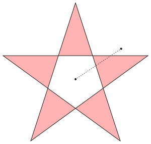
To see a strategy for Betty, consider the following diagram:
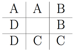
Betty’s strategy is simple: place an O in one of the squares marked A, one marked B, one marked C, and one marked D.
Note that this is always possible. Even if Clyde does not play in the center on his first move, he can only occupy one square labelled A, B, C, or D. Then Betty places her O on the other square with the same letter. If Clyde does begin in the center, then Betty has her choice of first move.
Since it is always possible — and since Betty only has four moves — these comprise all of Betty’s moves. But note that since Betty never has an O on two of the same letter, she can never get three-in-a-row on a side. Further, since Betty’s strategy never involves a move in the center, she can never get three-in-a-row in a line going through the center square. This means that Betty can never lose!
So if the two players play their best games, then Nic-Nac-No ends up in a draw. And while these strategies do indeed work, I would welcome someone to find simpler strategies.
I’ll leave you with another version of Tic-Tac-Toe to think about. Here are the rules: if during the game either play gets three-in-a-row, then X wins. If at the end, no one has three in a row, then O wins. Does X have a winning strategy? Does O? Note that in this game, there cannot be a draw! I’ll give you the answer in my next installment of Beguiling Games….


![[OP]\cdot[OP']=1,](https://s0.wp.com/latex.php?latex=%5BOP%5D%5Ccdot%5BOP%27%5D%3D1%2C&bg=ffffff&fg=333333&s=0&c=20201002)
![[AB]](https://s0.wp.com/latex.php?latex=%5BAB%5D&bg=ffffff&fg=333333&s=0&c=20201002) denotes the distance from A to B. Feel free to reread the previous two posts on inversive geometry for a refresher (here are links to the
denotes the distance from A to B. Feel free to reread the previous two posts on inversive geometry for a refresher (here are links to the  Points on a ray drawn from the origin through P will then have coordinates
  where
where  Thus, we just need to find the right
  so that the point
  satisfies the definition of an inverse point.
 and
and  if you substitute
  everywhere you see
  and substitute
  everywhere you see
  From our previous work, we know that the inverse curve must be a circle going through the origin.


 being the origin with coordinates
  ?
? translate to the point
  so that the point

 about the point
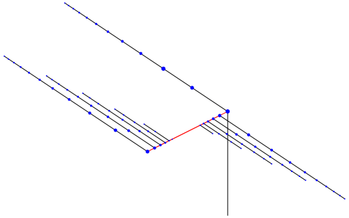
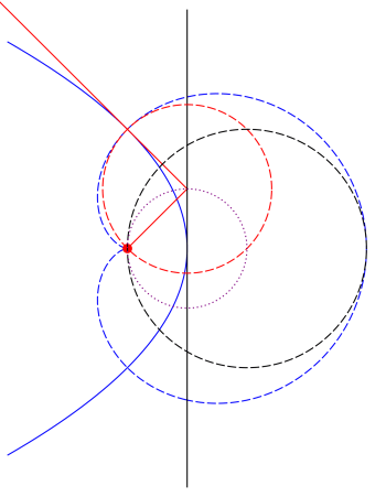
 inverted about a series of equally spaced points along the line segment with endpoints
  and
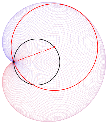
and  This might seem a little arbitrary, but it takes quite a bit of experimentation to find a set of points to invert about in order to create an aesthetically pleasing image.


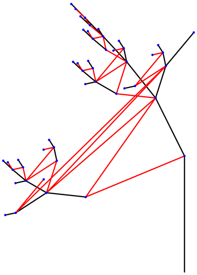
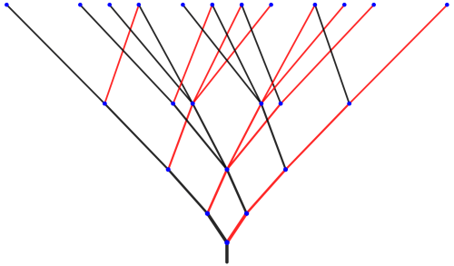
 and that which generate the red branches by
  you will observe behavior like that in the above tree if
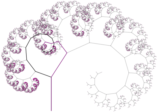
 is a scaled rotation by 60°. This is what produces the spirals of red branches emanating from the nodes of the tree.